1. Introduction

Convolutional Neural Networks (CNNs) have gained attention in recent years for their ability to perform complex machine learning tasks. Followed by winning the 2012 ImageNet competition, CNNs have demonstrated superior results in a wide range of fields including image classification, natural language processing and automotive. In addition to high accuracy in object recognition, systems using CNNs are more robust and resilient to noise in the inputs when compared to conventional algorithmic solutions. However, the enormous amount of computing power required by CNNs poses a great challenge to software as well as architecture engineers. The most time-consuming operation in a CNN is the convolution operation, which takes up over 90% of the total runtime. Therefore, the convolution operation becomes one of the most important concerns when implementing CNNs.

GPGPUs have demonstrated superior performance on CNN by exploiting the inherent computation parallelism. Due to the scaling architectures as well as ease-of-programming environment, GPGPUs are among the most widely adopted platforms for CNN. However, it is not a trivial task to have an efficient CNN design on a GPGPU. To achieve superior performance, a design involves careful concerns between exposing the massive computation parallelism and exploiting data reuse in complex data accesses.

This paper is an extension of work originally presented in ICASI 2017 [1]. In this paper, we perform a series of qualitative and quantitative studies on both the programming techniques and their implications on the GPU architecture. The observations reveal comprehensive understanding on the correlation between the design techniques and the resulting performance.  There exist several frameworks and libraries that provide solutions to performing convolution on GPGPUs, such as cuDNN [2], Caffe [3], fbfft [4], and cuda-convnet2 [5]. Among the existing solutions, cuda-convnet2 is one of the widely used open-source implementations that enable superior performance on a variety of CNN schemes [6]. It employs design techniques and optimization strategies mainly for NVidia GPGPU architectures. However, while providing a solid implementation, cuda-convnet2 lacks comprehensive analysis on its design techniques and decisions. The analytical discussion and quantitative proof behind the design criterion, such as choosing proper dimensions to parallelize, are not well studied. In addition, current GPGPUs are not designed specifically for convolution. There exist potential architecture enhancements that could significantly enhance the computation efficiency with minor hardware and software cost.

Figure 1: Convolution in CNN

This paper performs a series of qualitative and quantitative studies on both the programming techniques and their implications on the GPU architecture. The studies focus on the widely adopted NVidia GPGPU architecture and CUDA programming environment. The observations reveal comprehensive understanding on the correlation between the design techniques and the resulting performance. Based on the analyses, we pinpoint the two major performance bottlenecks of CNN on GPGPU: performing computation and loading data from global memory. Software and hardware enhancements are proposed in this paper to alleviate these issues. In the computation part, we demonstrate how to avoid excessive local memory accesses, the operations that severely degrade performance, by applying loop unrolling. We then propose two simple yet effective hardware accelerators to speed up the computation of the partial sums. In the data-loading part, we identify that a significant fraction of the time is spent on calculating addresses in the inner loops of CNN. We propose two software techniques to considerably reduce the computation. A low-cost address generator is then introduced to speed up the address calculation. Experimental results on a cycle-accurate GPGPU simulator, GPGPU-sim [7], have demonstrated up to 4.4x performance enhancement when compared with the original cuda-convnet2 design.

The rest of the paper is organized as follows. Section 2 discusses the implementation of the convolution kernel. The techniques of exposing parallelism and data reuse will also be discussed in Section 2. Section 3 and 4 describe the proposed software and hardware improvements to the convolution kernel. Section 5 discusses previous related works and Section 6 presents the conclusions.

2. Implementing Convolution on GPGPU

 2.1 Convolution in CNN

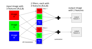
 Convolution is the basic building block as well as the most time-consuming operation in CNNs. The convolution operation in CNN does more than just convolving two 2D matrices. It takes a set of trainable filters and apply them to the input images, creating one output image for each input image. Each input image consists of one or more multiple feature maps, which means that every pixel in an image contains several features. For example, each pixel in an RGB picture contains three features: red, green and blue. Each filter also has the same number of features that correspond to the input images. When applying the filters to an input image, the filters are convolved across the width and height of the image, and the product of each feature is summed up to produce an output feature map. The number of features in each output image is therefore equal to the number of filters. Figure 1 illustrates an example of the convolution between one image and 2 filters with 3 features, producing one output with 2 features.

The high-level algorithm of the convolution operation in CNN is listed in Figure 2, where conv2 represents computing the 2D convolution between two 2D matrices. The inputs and outputs of the algorithm are all arranged in 4-dimensional arrays. Inputs to the algorithm are the image array images (image_count, height, width, image_features) and the filter array filters (image_features, filter_size, filter_size, filter_count). The output is the array outputs (image_count, height, width, filter_count). Each of the parameters used in the algorithm is described as below.

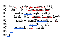Figure 2: Pseudocode of convolution operations

image count. This parameter is the size of input mini-batch. A mini-batch contains multiple independent input images to be processed. Each image in the mini-batch will be processed by the same set of filters to produce one output image.

width, height. These two parameters are the width and height of the input images. All input images in the mini-batch have the same size. In this paper, the size of output images is the same as the size of the input images.

image_features. This parameter indicates the number of features maps in an input image. This is also the number of feature maps in a filter.

filter_size. In the context of CNNs, filters are always square-shaped. Therefore, we use only one parameter, which is filter_size, to represent both the width and height of a filter. As a result, the number of pixels in a filter is (filter_size * filter_size).

filter_count. This parameter is the total number of filters. Because each filter produces an output feature map, filter_count is also the number of output feature maps.

2.2 Exploiting Parallelism and Data Reuse in Convolution

 This paper uses cuda-convnet2 [5] as the reference implementation of CNN on GPGPUs. Cuda-convnet2 is one of the widely used open-source implementations that enable superior performance on a variety of CNN schemes [6]. It employs design techniques and optimization strategies mainly for NVidia GPGPU architectures. This section will discuss how to implement the convolution algorithm efficiently with CUDA [8].

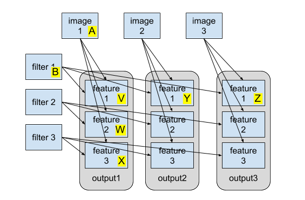Figure 3: The relation between the input data (images and filters) and the output images.

CUDA is a design environment for massively parallel applications. CUDA applications exploit parallelism provided by the GPGPU by breaking down the task into blocks containing the same number of threads. Functionally speaking, blocks are independent to each other. Although some of them may be assigned to the same computing tile (a.k.a. SM (Streaming Multiprocessor in NVIDIA GPU), the computing model dictates that one block cannot communicate with another. Threads in a block are assigned to the same computing tile so that they can communicate and share data. This computing model leads to two important design decisions: 1) which dimensions to parallelize; and 2) what data to share and reuse between threads with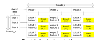in a block.

Figure 4: Configuration of threads in a block

Parallelizing one dimension means that the task is divided into smaller pieces by splitting at that dimension. For example, if we choose to parallelize the image_count dimension, computation for different images are divided into smaller tasks. In this case, each task is responsible for a small number of images. There are six dimensions in the inputs: image_count, image_features, width, height, filter_size and filter_count. A designer needs to decide which of these dimensions should be parallelized.

One limitation of the CUDA programming model is that different blocks cannot communicate with each other. Therefore, we can only parallelize dimensions that divide the problem into smaller independent tasks. In other words, outputs of each task should be stored separately without being combined into larger results. Based on this criterion, we will separately examine each of the dimensions to determine if it can be parallelized.

The dimension image_count represents the number of images. Because each image produces its own output independent of other images, we can parallelize the image_count dimension. The width and height dimensions can also be parallelized because computation of each output pixel is independent. Next, each filter produces its own output feature map, so the filter_count dimension can be parallelized. Now we are left with two dimensions to examine. The features dimension represents the number of feature maps in input images as well as filters. Because the results from different feature maps are summed to form a single output feature map (see Figure 1), we do not parallelize the feature dimension. Finally, we also do not parallelize filter_size because the products of filter pixels and image pixels are summed to form a single output pixel. To summarize, the dimensions that we are going to parallelize are image_count, width, height and filter_count.

The next step is to decide what data is reused and shared by different threads within a block. Figure 3 depicts the relation between the input data (images and filters) and the output images. Some input/output data set are labeled with capital letters for ease of explanation. The arrows in the figure indicates the input-output relation of the data. For example, the arrow pointing from A (image 1) to V (feature 1 of output 1) means that computation of V depends on A. From the figure we can see that different features in the same output image share the same input image (e.g. V, W, X all depend on A). Also, the same feature in different output images share the same filter (e.g. V, Y, Z all depend on B). These observations reveal some data-reuse opportunities.

 To benefit from reusing both images and filters, a block should load pixels of multiple images and filters from the global memory. The threads also need to efficiently reuse the loaded data. This can be done by arranging the threads into a 2D configuration as show in Figure 4. The total number of threads in a block is threads_x * threads_y, and each thread is responsible of computing a single output pixel. All threads have an x and y index, where the x index determines which image the thread uses and the y index determines the filter. By doing this, the kernel only needs to load threads_x image pixels and threads_y filter pixels to compute threads_x * threads_y outputs. Each loaded image pixel  is reused by threads_y threads, and each loaded filter pixel is reused by threads_x threads. As a result, this design reduces the memory access required to load the images to 1 / threads_y and that of the filters to 1 / threads_x.

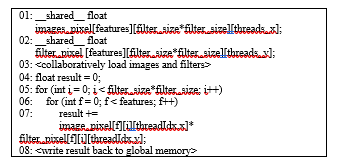Figure 5: High-level structure of the CUDA kernel

The high-level structure of the CUDA kernel is listed in Figure 5. Shared memory arrays are allocated to store the image and filter pixels to be reused. At the beginning, all threads work together to load the image and filter pixels required by the block. Then, each thread computes the output pixel it is responsible for. Finally, the computed results are written back to global memory.

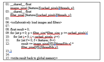Figure 6: Modified kernel that loads data in chunks

This kernel is functional, but there are some details that can be improved. The first one is that this kernel loads the entire filter into shared memory, resulting in higher shared memory usage. This can be improved by loading the filter pixels in fixed-size chunks instead of loading as a whole. Due to the commutativity and associativity of summation, the final result is equal to the sum of the partial result of each chunk. Now we can modify the program by adding a parameter cached_pixels to set the size of the chunk. The modifications are listed in Figure 6. Note that both images and filters are loaded in chunks, or tiles. This technique is normally referred as tiling. As listed in (1), the shared memory usage after tiling (SharedMem_tile) can be greatly reduced from the original cost (SharedMem_original).

Currently, each thread in the kernel computes only one output pixel. We can generalize the kernel to compute multiple output pixels per thread. An output pixel is computed from one image and one filter, so we will add two extra kernel parameters images_per_thread and filters_per_thread to make the kernel compute multiple output pixels. These two parameters decide how many images and filters should each thread use. Because each pair of image and filter generate one output pixel, the number of outputs of each thread is images_per_thread * filters_per_thread. The modification to the program is listed in Figure 7. By adjusting images_per_thread and filters_per_thread, we can make each thread compute multiple outputs and therefore reduce the total number of blocks for the same problem size. For example, if the original kernel (equivalent to the modified kernel with images_per_thread = filters_per_thread = 1) has N blocks in total, the new kernel with images_per_thread = filters_per_thread = 2 only has N/4 blocks.

This kernel is used as the baseline program on which we propose enhancements. In the next section, we will describe how we choose the input sizes to use in our experiments.

2.3 Choosing the Input Size for Experiments

GPGPU-sim can obtain detailed execution behavior of CUDA programs on a GPU architecture similar to GTX-480. However, performance simulation in GPGPU-sim is very slow compared to a physical GPU. For example, a program that takes 100ms on an NVidia GTX480 can take up to 3 hours when running on GPGPU-sim. With such long simulation periods, changes to the program or the simulator itself cannot be quickly tested. Therefore, we think it is beneficial to reduce the size of the input dataset for shorter simulation time. But reducing the input data size, if done improperly, might produce inaccurate simulation results that deviates from the behavior of the original data. In this section, we will discuss a way to choose the size of the reduced data.

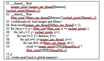Figure 7: Modified kernel with multiple output in each thread

Computation in CUDA is broken down into independent blocks. Each block is assigned to a streaming multiprocessor (SM) so that every thread in the block can be run concurrently via fine-grain context switching of warps (groups of 32 threads). Also, each SM is capable of executing multiple blocks at the same time. On GTX480, the maximum number of blocks that a SM can run concurrently is limited by the following limiting factors:

1. An SM has 32768 registers.
2. An SM has 48kB of shared memory.
3. There should be no more than 8 blocks assigned to the same SM at the same time.

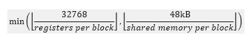
Each thread in a block has its own set of registers, so the number of registers used by each block is block size×register per thread. The limitation of blocks per SM due to the limiting factor 1 mentioned above is

Another limitation is the size of shared memory. Because an SM only has 48kB of shared memory, the limiting number of blocks per SM due to limiting factor 2 is

At last, due to scheduler hardware limitations (limiting factor 3), a SM can only run at most 8 blocks concurrently. Concluding (2), (3) and the hardware limitation, the actual maximum number of blocks per SM can be obtained by (4).

(4)

In GTX480, there are 15 SMs. If each SM can run eight blocks in parallel, then the GPU can run 120 blocks concurrently. While using very large datasets, the total number of blocks will be much larger than 120 so that most of the time, all SMs on the GPU is doing some work. However, if the reduced dataset has less than 120 blocks, then some of the SMs on the GPU will be idle all the time, making occupancy lower than it should have been in larger datasets. Also, if the number of blocks is slightly more than 120 blocks, the GPU will execute the first 120 blocks in its full capability, and then execute the remaining blocks using only some of the SMs while leaving other SMs idle. This also makes measurements inaccurate in the same way.

Therefore, it is preferable to adjust the reduced data size so that blocks fill in all SMs during the entire simulation period. In other words, the total number of blocks divided by the maximum number of concurrent blocks should be a whole number or slightly less than a whole number (ex. 1.99). By reducing the data size like this, measurements will be closer to that of larger data sets.

Input parameters		Kernel parameters
image_count	128	images_per_thread	4
image_width	5	filters_per_thread	4
image_height	6	threads_x	16
image_features	3	threads_y	4
filter_count	32	cached_pixels	4
filter_width, filter_height	32

Table 1: Parameters used in the experiments

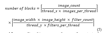
The actual input data size and kernel parameters we use in the experiment are listed in Table 1. According to these parameters, we can compute the total number of blocks using (5).

After compiling this program, the compiler outputs the following information:

1. Each thread uses 28 registers.
2. Each block uses 3900 bytes of shared memory.

Now we compute the number of blocks per SM. The limitation caused by registers is

Because both (6) and (7) exceed the hardware limitation of eight blocks per SM, maximum numbers of blocks per SM in this case is 8. Multiplying with the total numbers of SMs on GTX480, we get 8×15=120 blocks that can be executed on the GPGPU in parallel. Since there are exactly 120 blocks to be executed, all the blocks can be run in parallel without any SM stalling.

2.4 Summary of Design Concerns

In this section, we discussed an implementation of convolution in CUDA step-by-step. This convolution kernel employs a 2D block configuration to enable sharing of onboard data between threads through the shared memory, reducing accesses to the global memory. The kernels are also parameterized to enable adjusting the amount of work done by each thread. We also explained how we choose a relatively small input size that utilize all SMs. This method of choosing input sizes reduces the error of the experiment results caused by idle SMs. In all the following experiments, we will use the input sizes listed in Table 1.

According to simulation using GPGPU-sim, we identified that the two bottlenecks of the convolution kernel are computation of partial sums and loading of image and filter data. The following two sections, Section 3 and Section 4, will elaborate the proposed software and hardware improvements to speed up these two bottlenecks.

3. Accelerating Computation Part

The result of profiling the baseline implementation is shown in Figure 8. According to the profiling result, the most time-consuming part in the entire kernel is the computation part, which takes up over 97% of the overall runtime. In this section, we will focus on reducing the computation cost by various techniques including software and hardware modifications.

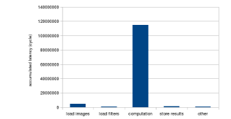Figure 8: Initial Performance Breakdown

3.1 Avoid Local Memory Access

In order to improve the performance of the computation part, we need to understand what is responsible for its relatively long latency. Instruction-level breakdown of the profiling result listed in Figure 9 reveals that the latencies of instructions accessing local memory are orders of magnitude greater than other instructions. In this section, we will discuss why there is local memory accessing in the code and how can we avoid it.

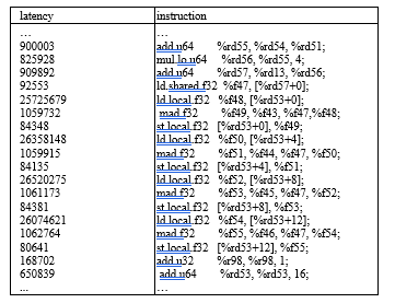Figure 9: Local memory access latency

3.1.1   Local Variables in CUDA

Before going into discussion, we will first briefly introduce how local variables (also known as automatic variables) are handled in NVidia GPGPUs. In the CUDA programming language, local variables are normally placed in the stack frame of the current function call. But compilers are also allowed to put them in registers if the architecture permits. Execution stack of CUDA threads are placed in a special memory space called local memory. Local memory resides in the global memory but is partitioned and allocated to each thread. Each thread can only see its own copy of local memory. Because global memory is much slower than registers, it is often preferable to put local variables in registers instead of 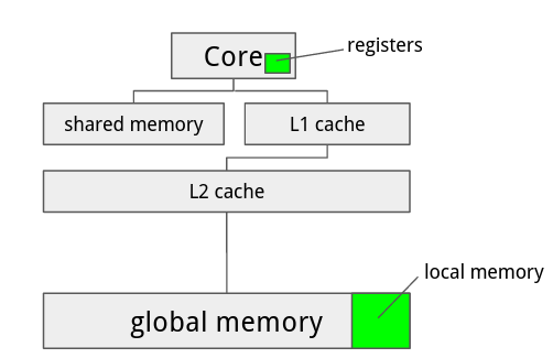local memory.

Figure 10: Registers and Local Memory

However, there are two limitations in CUDA regarding the use of registers. One limitation is that Fermi GPGPUs only have 32768 register in each core, so the total number of registers used by all threads in a block cannot exceed 32768. This limitation is less of a problem in convolution because the number of threads per block is relatively small (less than 100), and the number of register required for each thread is around 60. The other limitation is that registers have no addresses. This implies that an array can be put in registers only if no indexing is performed on them.

3.1.2 Loop Unrolling

In the convolution kernel, the partial sums computed by each thread are stored in a local array and accumulated over all pixels as shown in Figure 11. The loop counter f and g are used with the subscript operator to access the array element for each image and filter. In this case, the compiler needs to put the array in local memory because registers cannot be indexed. This will cause the GPU to access global memory in every iteration of the inner loop.

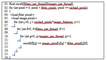Figure 11: Local Array in the Convolution Kernel

It can be seen in the figure that the overall latency is dominated by local memory access (highlighted in boldface). The bottleneck can be totally avoided if the array elements are put in registers instead of local memory. However, the compiler cannot put the array in register because the array needs to be dynamically indexed.

One way to get around this limitation is to apply loop unrolling, which effectively eliminates all dynamic indexing on the array by expanding the loop and replacing the indices with constants. As long as the array is not dynamically indexed, the compiler can allocate registers for the array elements.

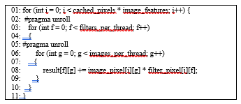Figure 12: Applying Loop Unrolling

Loop unrolling in CUDA can be enabled by setting up the preprocessing hint during compilation. A directive #pragma unroll is provided to let the programmer issue unrolling hints so that the compiler knows which loops should be unrolled. Using the unroll directive, we can apply loop unrolling to the original program (shown in Figure 12). By using loop unrolling on the two inner-most loops, the `result` array is expanded into multiple independent registers. As a result, the inner loop no longer requires local memory access. As shown in the profiling result in Figure 13, latency of local memory accesses is completely eliminated after unrolling the loop.

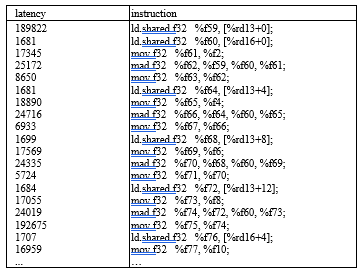Figure 13: Profiling result after applying loop unrolling

Before applying loop unrolling, it takes 524k cycles for the program to finish. The letter k is a postfix indicating 1,000. After applying loop unrolling, the number of cycles is reduced to 148k, resulting in a 71% improvement on the overall performance. The latency breakdown in Figure 14 shows that the computation part is dramatically improved by loop unrolling.

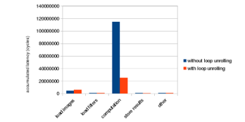Figure 14: Loop unrolling performance improvement

3.2 Adding Inner Product Engine

The computation part (shown in Figure 15) is still the bottleneck even after applying loop unrolling, taking up about 69% of the overall execution time. Looking at the loop as a whole, what it does is computing the product between each image and filter pixel and sum them together. The partial sums are then accumulated in the array `result`.

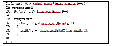Figure 15: Computation loop

If we exchange the order of the outmost loop with the two inner loops in Figure 16, the inner loops (Line 05 to Line 11) becomes an inner product operation between the two arrays. This modification does not change the behavior of the original function because there is no dependency between each loop iteration. Since the two outer loops are unrolled, the inner product becomes the only bottleneck.

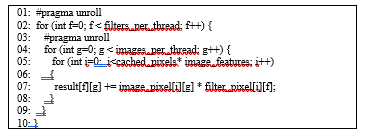Figure 16: Inner product in the computation loop

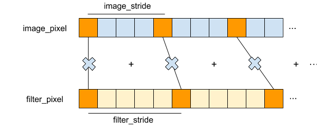Figure 17: Inner Product

To reduce the bottleneck, we propose adding a hardware inner product accelerator to the cores, one unit for each thread. The accelerator loads pairs of image and filter pixels from shared memory, compute the product of each pair, and then sum all the products together. The program passes the starting addresses and strides of both arrays and the number of elements to the accelerator. These arguments are then stored in the internal registers of the accelerator and are reused until their values are changed again. The final result is also stored in the unit and can be retrieved in the program.

The hardware architecture of the inner product accelerator unit is shown in Figure 18. For each iteration, it loads two elements from shared memory and accumulate the product of them to a register. It requires one multiplier, one adder and a register to store the partial results. In the actual implementation, the multiplier and adder can be fused into a fused multiply-add (FMA) circuit. We assume that it requires 2 cycles to load the two elements from shared memory, and the latency of the FMA is also assumed to be 2 cycles. A 2-stage pipeline can then be used to repeatedly load elements and compute FMA. In our work, we model the latency of the inner product unit as 2 * N, where N is the number of elements to compute.

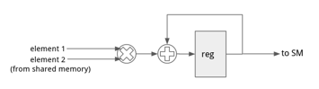Figure 18: Inner Product Unit

Modeling the accelerator requires modifying both GPGPU-sim and the application. We modeled the inner product accelerator in GPGPU-sim by intercepting memory access to specific addresses. We modified the load (ld) and store (st) handlers to check if the source or target address matches any of the designated addresses. List of the addresses we use and their functions are listed in Table 2. If the address matches, the original memory access is skipped and the corresponding function of the accelerator is performed. For example, as soon as the thread writes 16 to address 0xffffffc8, GPGPU-sim sets the stride register of the accelerator to 16.

Table 2: Addresses used by the inner product engine

address	direction	function
0xffffffc0	write	address of image array
0xffffffc8	write	stride of image array
0xffffffd0	write	address of filter array
0xffffffd8	write	stride of filter array
0xfffffff0	write	number of elements
0xfffffff8	read	start computing and retrieve the result; stall the thread for N cycles

To use this inner product accelerator, the application needs to use the addresses to manipulate the registers inside the accelerator. First, the application should pass the starting address of the image and filter array to 0xffffffc0 and 0xffffffd0 respectively. The image stride is threads_x * images_per_thread, and the filter stride is threads_y * filters_per_thread. These two values are constant as the dimensions of the arrays are known in compile time, so it is only necessary to write them once at the beginning of the kernel. The fifth parameter, number of elements, is also known in compile time and only needs to be write once. Finally, after all parameters are set, the program needs to read from address 0xfffffff8 to retrieve the result of the inner product. The modified program is listed in Figure 19.

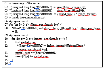Figure 19: Program modified to use the inner product engine

The profiling result of the modified program is listed as follows in Figure 20. As shown in the figure, the computation part is improved by 88% and results in 66% improvement on the overall performance. The bottleneck of the program is no longer the computation part.

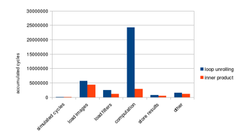Figure 20: Loop unrolling performance improvement

3.3 Outer Product Engine

In this section, we will discuss an alternative way to accelerate at the computing part. The two inner loops (shown in line 03~09 in Figure 21) can also be viewed as computing the products of each pair of elements in image_pixel[i] and filter_pixel[i]. This operation is called the outer product, which can be represented as multiplying a column matrix with a row matrix as shown in the figure. Inputs to the outer product are two arrays image_pixels[i] and filter_pixel[i], each with length images_per_thread and filters_per_thread. Each element in the first array is multiplied with each element in the second array, producing a total of images_per_thread * filters_per_thread numbers. The outer product is performed cached_pixels * image_features times, and the output of each time is accumulated to produce the partial sums.

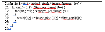Figure 21: Outer product in the computation loop

We propose an accelerator to speed up the computation of the outer product. The accelerator has at least images_per_thread * filters_per_thread internal registers to store the computed partial sums. It loads two arrays, compute the product of each pair of elements, and accumulate the results to the internal registers. Values of the registers can be read or reset to zero by the program.

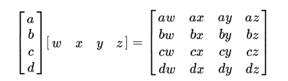Figure 22: Outer product

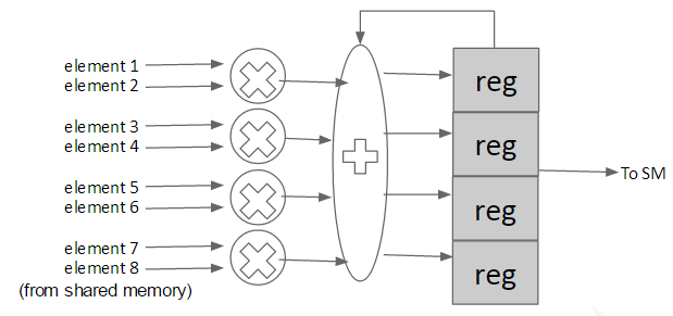Figure 23: Outer Product Unit

The hardware architecture of the outer product accelerator unit is shown in Figure 23. For each iteration, it loads four elements from image array and one element from filter array multiply them to a register, and the adder adds previous partial sum to the original register. It consumes four multiplier, one adder and number of image array * filter array registers to save the partial results. Suppose the multiplier requires 1 cycle to produce the result, storing result to register and loading pixel from shared memory also consumes 1 cycle. Then, a 3-stage pipeline can be applied to repeatedly load elements, compute outer product and store results. In our implementation, we model the latency of the outer product unit which assume that the accelerator can load one pixel from the shared memory each cycle. It will need to preload some pixels from the image array before using a 3-stage pipeline, and the number of preloaded pixels depends on image array length. Therefore, we can assume that the total latency of the accelerator is image array length + (2*N)-2 ,where N is the number of elements to compute.

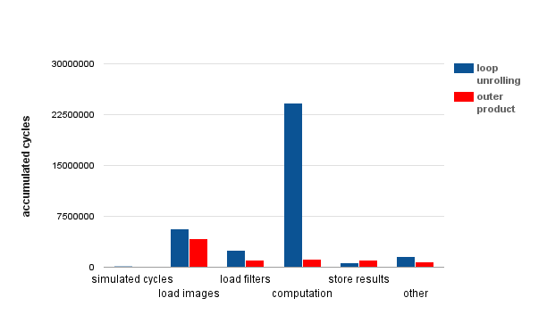Figure 24: Outer product performance improvement

4. Accelerating Data-Loading

After applying the improvements described in Section IV, the computation part is improved a lot. As illustrated in Figure 25, the data-loading part, including loading of images and filters, becomes the bottleneck of the program.

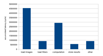Figure 25: Performance breakdown after improvements

The data-loading part is responsible for loading image and filter pixels from global memory to shared memory. It is composed of deeply nested control structures of loops and conditionals. The control structures themselves also take time to execute, especially for the inner loops. Any subtle overhead inside inner loops can build up and become major bottlenecks. In this section, we propose two software approaches to reduce the overhead inside inner loops. We also propose a hardware accelerator to speed up address calculation in the image-loading part.

4.1  Strength Reduction

One of the major bottlenecks in inner loops is the computation of array indices for each iteration. In the data-loading loops, array indices in inner loops can contain complex arithmetic expressions that translates into larger number of instructions. Because the arithmetic instructions are executed in the inner loops, latencies of them can quickly build up and become a major bottleneck.

Take the program in Figure 26 as an example. To compute the array index for images, it needs to compute two multiplications and two additions for each iteration (line 4). If we work out the total number of operations, we will find that the program needs to carry out image_features * images_per_thread multiplications and additions in total.

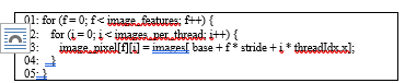Figure 26: Arithmetic operation in the inner loop

We propose a method based on strength reduction to improve the performance of this program. This method takes advantage of the fact that some arithmetic operations can be reduced to successive simpler operations. For example, multiplication can be done with repeated addition of the multiplier. Instead of computing the multiplication in each iteration, we can use a separate counter variable idx to accumulate the index throughout the entire loop and update it according to the following rule.

The arithmetic expression for computing the array index can be broken down into 3 parts:

1. loop invariants (terms that does not change throughout the nested loops)
2. multiples of the outer loop counter f
3. multiples of the outer inner loop counter i

Terms belonging to Part a is constant with respect to both the inner and outer loops. Therefore, the term `base` is used to initialize idx before entering the loops. Part b contains the term f * stride, whose value increases by stride whenever f is incremented. Therefore, stride is added to idx at the end of the outer loop. Part c contains the term i * threadIdx.x. The value of this term goes from 0 to (images_per_thread-1) * threadIdx.x in the inner loop and returns to zero again. Therefore, we will first save the value of idx before entering the inner loop, increment idx in each iteration, and restore idx after leaving the inner loop. The resulting program is listed in Figure 27.

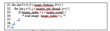Figure 27: Applying strength reduction

In this transformed program, it only needs to compute one addition for each iteration in the inner loop and one addition for each iteration in the outer loop. In total, we get image_features * (images_per_thread+1) additions. The total number of operations is cut in half compared to the original program, so the modified program should run faster in the data-loading part. Profiling results in Figure 28 supports this prediction by showing that the performance of the image-loading and filter-loading parts are improved significantly. The impact of strength reduction is 25.9% on the overall performance.

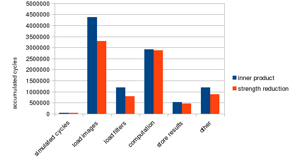Figure 28: Strength reduction performance improvement

4.2   Extract Conditionals

In addition to strength reduction, we also identified another useful optimization strategy in the data-loading loop. The idea is to prevent unnecessary condition checks in inner loops by checking whether the conditional is necessary in the loop before entering the loop. To illustrate the case, consider the following code snippet taken from the convolution kernel:

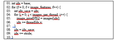Figure 29: Boundary checking in the data-loading loop

In the inner-most loop, it checks whether the index of image to load (image_index + i) is within bounds and only load the image if so. Because the total number of image is not always a multiple of images_per_thread, the boundary condition check is necessary here to ensure that the index to load is within bounds. However, checking for the boundary condition every time in an inner loop degrades performance. To eliminate redundant checks in inner loops, the loop is duplicated and modified into two variants: one with boundary checking, and the other without them. Without the checking overhead, the one without boundary checking will run faster. The problem we are left with is how to choose between these two variants.

Because the loop variable i is always less than or equal to images_per_thread – 1, image_index + i will always be less than or equal to image_index + images_per_thread – 1. If given image_index + images_per_thread – 1 < image_count, we will automatically get image_index + i < image_count. In other words, if image_index + images_per_thread <= image_count, there is no need to check for the boundary condition. As a result, we will choose the faster loop without boundary checking if image_index + images_per_thread <= image_count, or the slower loop otherwise. The resulting code is listed in Figure 30.

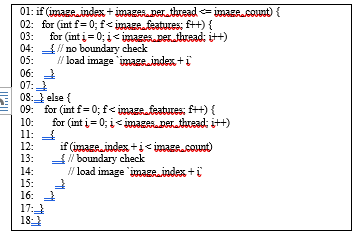Figure 30: Reduced boundary check code

Profiling result before and after applying this technique is shown in Figure 31. This technique improves the overall performance by 2.6% compared to the previous version using only strength reduction.

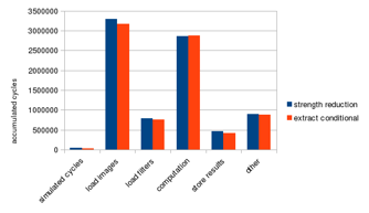Figure 31: Extract conditionals performance improvement

4.3   Index Conversion Accelerator

In the data-loading part of the convolution kernel, filter and image pixels are loaded to shared memory one after another. Before loading each pixel from global memory, the program must compute the index of the pixel in the input arrays. In each iteration of the loop, the program first loads several filter pixels. While loading the filter, there is no need to compute the index because the loop counter itself represents the index of the filter pixel to load. However, for each filter pixel, it is still necessary to load the corresponding image pixel. Computing the index of image pixels is more involved. Sometimes the filter pixel is placed outside the image and doesn’t overlap with any pixel in the input. When this happens, the loaded image pixel should be set to zero because zero-padding is used outside the edges of the image. If the filter pixel is placed within the image, the filter pixel index should be converted into the image pixel index, which is then used to load the image pixel from global memory.

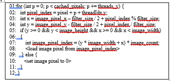Figure 32: Index conversion in the data-loading loop

Computing the image pixel index and checking for the boundary condition takes up about 1/3 of the image-loading time. Therefore, we propose adding an accelerator to speed up this two tasks at the same time. Before describing what this accelerator should do, we will first look at the code to convert filter pixel index to image pixel index.

From the code listed above, we can see that there are three steps involved in converting filter pixel index to image filter index. The first step is break down filter pixel index to its x and y component and offset the coordinates by the location of the kernel. Then, boundary check is performed on the (x, y) point to ensure that there is a corresponding pixel in the input. Finally, the (x, y) is converted to the image pixel index. These steps are translated to tens of instructions and slows down the program.

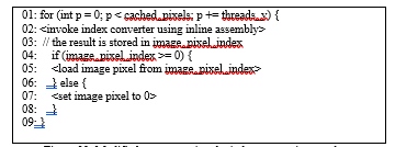Figure 33: Modified program using the index conversion accelerator

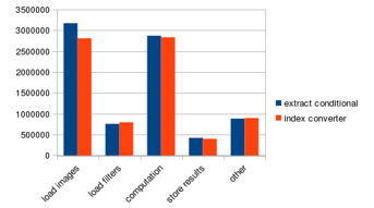Figure 34: Index converter performance improvement

We propose adding a hardware accelerator to do the index conversion. The accelerator we propose will do the three steps altogether in one instruction. If the (x, y) point is within bounds, it returns the index of the image pixel. Otherwise, it returns -1. We implement the accelerator in GPGPU-sim as an instruction and use inline assembly in the convolution kernel to invoke the instruction. The modified program is listed in Figure 33. The performance improvement of using the index converter is listed in Figure 34. The overall performance is improved by 5%.

5. Related Work

Accelerating convolutional neural networks is a very popular research topic. Accelerators have been developed in different hardware technologies. Eyeriss [9][15] developed by Yu-Hsin Chen et al. is an ASIC CNN accelerator that can run AlexNet at 35fps with only 278mW of power consumption. There are other ASIC accelerators proposed to exploit the redundancy of CNN networks [16][17][18]. Cheng Zhang [10] implemented a CNN accelerator on FPGA and achieved 61.62 GFLOPS under 100MHz clock frequency. He also proposed an analytical design scheme using the roofline model.

The GPGPU is also a widely-used platform for CNN. NVidia developed a software library named cuDNN [2] that uses GPGPU to speed up convolution. When integrated with the Caffe framework, it can improve the performance by up to 36%. However, the cuDNN library is proprietary and cannot be studied by the community. The fbfft library [4] also uses GPGPU to speed up CNN, but it employs a different algorithm (FFT) to compute convolution. Cuda-convnet2 is an efficient implementation of CNN for NVidia GPGPU. It is by far the fastest open-source CNN implementation. However, it lacks analysis on the techniques it uses to improve the performance.

6. Conclusion

This paper describes an implementation of the convolution operation on NVidia GPGPU and analyze the techniques in the implementation. We propose software and hardware enhancements to the program to speed up the computation of partial sums and loading the input data, which are the two major bottlenecks. The experiments have shown that the proposed modifications have achieved 4.4x speedup compared with the baseline implementation.

1. Lin, C.-H.; Cheng, A.-T.; Lai, B.-C.; “A Software Technique to Enhance Register Utilization of Convolutional Neural Networks on GPGPUs,” IEEE International Conference on Applied System Innovation, May 2017. http://ieeexplore.ieee.org/document/7988499/
2. Chetlur, S., Woolley, C., Vandermersch, P., Cohen, J., Tran, J., Catanzaro, B., & Shelhamer, E. (2014). cudnn: Efficient primitives for deep learning. arXiv preprint arXiv:1410.0759. https://arxiv.org/abs/1410.0759
3. Jia, Y., Shelhamer, E., Donahue, J., Karayev, S., Long, J., Girshick, R., … & Darrell, T. (2014, November). Caffe: Convolutional architecture for fast feature embedding. In Proceedings of the 22nd ACM international conference on Multimedia (pp. 675-678). ACM.
4. Vasilache, N., Johnson, J., Mathieu, M., Chintala, S., Piantino, S., & LeCun, Y. (2014). Fast convolutional nets with fbfft: A GPU performance evaluation. arXiv preprint arXiv:1412.7580. https://arxiv.org/abs/1412.7580
5. Alex Krizhevsky. cuda-convnet2. https://code.google.com/p/cuda-convnet2/, 2014. [Online; accessed 23-January-2015].
6. Lavin, A. (2015). maxDNN: an efficient convolution kernel for deep learning with maxwell gpus. arXiv preprint arXiv:1501.06633. https://arxiv.org/abs/1501.06633
7. Bakhoda, A., Yuan, G. L., Fung, W. W., Wong, H., & Aamodt, T. M. (2009, April). Analyzing CUDA workloads using a detailed GPU simulator. In Performance Analysis of Systems and Software, 2009. ISPASS 2009. IEEE International Symposium on (pp. 163-174). IEEE. http://ieeexplore.ieee.org/abstract/document/4919648/
8. Nickolls, J., Buck, I., Garland, M., & Skadron, K. (2008). Scalable parallel programming with CUDA. Queue, 6(2), 40-53.
9. Chen, Y. H., Krishna, T., Emer, J., & Sze, V. (2016, January). 14.5 Eyeriss: An energy-efficient reconfigurable accelerator for deep convolutional neural networks. In 2016 IEEE International Solid-State Circuits Conference (ISSCC) (pp. 262-263). IEEE. http://ieeexplore.ieee.org/document/7738524/
10. Zhang, C., Li, P., Sun, G., Guan, Y., Xiao, B., & Cong, J. (2015, February). Optimizing fpga-based accelerator design for deep convolutional neural networks. In Proceedings of the 2015 ACM/SIGDA International Symposium on Field-Programmable Gate Arrays (pp. 161-170). ACM. https://dl.acm.org/citation.cfm?id=2689060
11. Krizhevsky, A., Sutskever, I., & Hinton, G. E. (2012). Imagenet classification with deep convolutional neural networks. In Advances in neural information processing systems (pp. 1097-1105). https://dl.acm.org/citation.cfm?id=2999257
12. Simonyan, K., & Zisserman, A. (2014). Very deep convolutional networks for large-scale image recognition. arXiv preprint arXiv:1409.1556. https://arxiv.org/abs/1409.1556
13. Chen, T., Du, Z., Sun, N., Wang, J., Wu, C., Chen, Y., & Temam, O. (2014, February). Diannao: A small-footprint high-throughput accelerator for ubiquitous machine-learning. In ACM Sigplan Notices (Vol. 49, No. 4, pp. 269-284). ACM. https://dl.acm.org/citation.cfm?id=2541967
14. Cavigelli, L., Magno, M., & Benini, L. (2015, June). Accelerating real-time embedded scene labeling with convolutional networks. In Proceedings of the 52nd Annual Design Automation Conference (p. 108). ACM. http://ieeexplore.ieee.org/document/7167293/
15. -H Chen, T. Krishna, J. S. Emer, and V. Sze, “Eyeriss: An energy-efficient reconfigurable accelerator for deep convolutional neural networks,” IEEE Journal of Solid-State Circuits, 2017.
16. Kim, J. Ahn, and S. Yoo, “A novel zero weight/activation-aware hardware architecture of convolutional neural network,” in Design, Automation, and Test in Europe (DATE), 2017.
17. Parashar, M. Rhu, A. Mukkara, A. Puglielli, R. Venkatesan, B. Khailany, J. Emer, S. W. Keckler, and W. J. Dally, “SCNN: An accelerator for compressed-sparse convolutional neural networks,” in 44th Annual International Symposium on Computer Architecture (ISCA), 2017, pp. 27–40.
18. Zhang, Z. Du, L. Zhang, H. Lan, S. Liu, L. Li, Q. Guo, T. Chen, and Y. Chen, “Cambricon-X: An accelerator for sparse neural networks,” in 49th IEEE/ACM International Symposium on Microarchitecture (MICRO), 2016.

(Click to view)

(Click to view)