1. Introduction

Process industries were recently observing significant changes, due to the need to increase the automation features. This requirement is strictly related to the increasingly stringent environmental and pollution standards that are connected to the need to improve the energy efficiency level [1]. For this purposes, Advanced Process Control (APC) solutions are receiving the attention of process engineers [2]. Significant benefits can be obtained with respect to standalone controllers, both from process control and energy efficiency achievement and improvement point of view [3,4]. The magnitude of these results is directly tied to the amount of energy required for the considered processes.

Steel industry represents a high-energy intensive process industry: it is characterized by different complex phases that have to be carefully managed. Figure 1 briefly depicts the production chain of a steel industry [5]. Initially, raw materials (e.g. waste materials) are processed (Figure 1, Raw Materials Processing Phase) in order to obtain steel bars at an intermediate stage of manufacture, e.g. billets. Billets are then introduced in a reheating furnace in order to be suitably reheated (Figure 1, Reheating Phase). There are different typologies of reheating furnaces, distinguished by the furnace movement methodology: for example, in a pusher type reheating furnace, billets are moved along the furnace through the action of pushers. Billets can enter the furnace at different temperatures. In the case study that will be proposed in the present paper, i.e. a pusher type billets reheating furnace located in an Italian steel plant, the billets inlet temperature range is 20 [°C] – 700 [°C]. Through the combustion reactions triggered by some burners, i.e. air/fuel burners, billets are exposed to heating reactions during their path along the furnace. The billets must be reheated in order to fulfill the specifications required for the subsequent plastic deformation phase (Figure 1, Rolling Phase). In the proposed case study, a range example for billets discharge (furnace outlet) temperature is 1000 [°C] – 1100 [°C]. From the final phase, the finished products, e.g. iron rods or tube rounds, are obtained.

Figure 1.   General production chain of a steel industry.

In a steel industry, the previously described Reheating Phase represents a crucial phase from an energy efficiency and products quality point of view [6]. In order to guarantee the desired trade-offs between the conflicting challenges of the steel industry Reheating Phase, i.e. energy saving and environmental impact decreasing versus product quality and production maximization, different approaches have been proposed in the control literature, ranging from classic to innovative techniques. In [7], a nonlinear optimization problem is formulated through a genetic algorithms approach; the minimization of fuel cost and the satisfaction of a desired discharge temperature represent the control objectives. In [8], two models and two related tracking control systems are proposed. In [9], a mixed neural network/heat transfer model approach is exploited, achieving an integrated intelligent control method. In [10], a nonlinear predictive approach is exploited for controlling a steel slabs continuous reheating furnace. A first principles mathematical model is developed that allows the controller to define the appropriate local furnace temperatures required for the achievement of the desired slabs discharge temperatures. The enormous potential of model-based control and optimization for steel reheating furnaces is described in [11], where one of the proposed control approaches is based on a transient nonlinear furnace model.

This paper is an extension of work originally presented in the 2017 6th International Symposium on Advanced Control of Industrial Processes (AdCONIP) [12]. In [12], the authors have presented an APC framework for the optimization of a pusher type billets reheating furnace (Reheating Phase) located in an Italian steel plant. Some details about the process features, the controller formulation and field results have been provided, highlighting the achieved benefits with respect to the previous control system, based on local temperature controllers managed by plant operators. In this paper, in addition to the previously reported literature analysis, additional aspects about the process modellization are provided. Furthermore, more details on simulation results are given through specific scenarios. Finally, results related to the installation of the developed APC system, denoted “i.Process | Steel – RHF”, on the Italian industrial plant are depicted and discussed, analyzing process control and energy efficiency aspects.

The paper organization is the following: Section 2 details the main process features, focusing on the control specifications and on the formulated process model. Details on the obtained relationships between the main process variables are provided. Section 3 depicts the control architecture, detailing the formulation of the two MPC modules. A significant plant scenario is reported
in Section 4, where a typical condition is simulated and managed with the activation of the developed APC system. In Section 5, results related to the installation on the Italian steel industry are reported, focusing on process control performances and on energy efficiency evaluation with respect to the computed baseline. Section 6 reports the conclusions.

2. Process description and modellization

This section reports the description of the considered case study, i.e. a pusher type billets reheating furnace located in an Italian steel plant. Furthermore, the formulated process model is described.

2.1.  Pusher Type Reheating Furnace

As previously described, a pusher type billets reheating furnace located in an Italian steel plant represents the case study that is proposed in this paper for the illustration of the main peculiarities of “i.Process | Steel – RHF” APC system. Figure 2 reports a synoptic of the developed Graphical User Interface (GUI) where a schematic representation of the considered reheating furnace is given. Note the three furnace areas: Preheating Area (green rectangle), Heating Area (yellow rectangle), Soaking Area (red rectangle). The main features of the furnace areas have been reported in Table 1. The furnace billets capacity is 136 (m_b=136); the billets are moved along the furnace based on the defined furnace production rate (up to 120 [t/h]). Billets enter the furnace through the Preheating Area (Figure 2, left side). In their path along this furnace area, they cross a unique zone (tunnel, 4.733 [m] length) that is not equipped with an own burners set. Subsequently, billets are moved towards the Heating Area that is constituted by zone 6 (3.477 [m] length), zone 5 (6.4 [m] length), and zone 4 (3.2 [m] length). All these furnace zones have air/fuel burners (Figure 2, yellow circles). Finally, billets enter the last furnace area, i.e. Soaking Area (Figure 2, right side). Three zones constitute this furnace area, characterized by an own burners set (Figure 2, red circles): zone 3 (4.546 [m] length), zone 2 (3.2 [m] length), and zone 1 (3.2 [m] length). Zone 2 and zone 1 are vertically disposed. Table 2 contains some billets features related disposed. Table 2 contains some billets features related to the considered case study.

Flowmeters detect air and fuel (natural gas) flow rates. The furnace zones temperatures are measured through thermocouples. Furnace and air pressures are measured by manometers placed near the furnace inlet. Billets temperature is measured by optical pyrometers only at the furnace inlet and after the billets furnace discharge (in the rolling mill area). Before the installation of “i.Process | Steel – RHF” APC system, no information was available about billets heating profile within the furnace. Plant operators managed the local Proportional Integral Derivative (PID) temperature controllers; they try to ensure the desired billets discharge temperature exploiting their experience and skills. However, due to the multivariable, nonlinear and time- varying characteristics of the considered process, the observed billets furnace discharge temperature was often higher than the minimum required temperature.

Through deepened process preliminary studies, significant energy efficiency margins (fuel specific consumption minimization) have been identified. For this reason, an APC

Figure 2.   Pusher type reheating furnace synoptic.

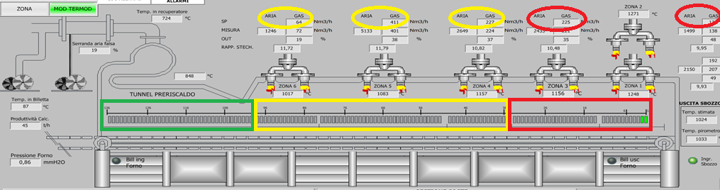
Table 1: Details of furnace areas

Area	Billets Number / Area Length	Temperature	Acronym [Units]
Preheating	38 / 4.733 [m]	Tunnel Temp.	Tun [°C]
Heating	64 / 13.077 [m]	Zone 6 Temp.	Temp6 [°C]
		Zone 5 Temp.	Temp5 [°C]
		Zone 4 Temp.	Temp4 [°C]
Soaking	34 / 7.746 [m]	Zone 3 Temp.	Temp3 [°C]
		Zone 2 Temp.	Temp2 [°C]
		Zone 1 Temp.	Temp1 [°C]

Table 2: Billets details

Billets Feature	Case Study Billets Feature Value
Mass	2.2815 [t]
Length	9 [m]
Section	0.2 [m] × 0.16 [m]
Inlet Temperature	20 [°C] – 700 [°C]
Discharge Temperature	1000 [°C] – 1100 [°C]

system customized for the analyzed process has been developed. In particular, as it will be described in Section 3, a Model Predictive Control (MPC) strategy based on linear models has been formulated [13-15].

2.2.  Process Modellization

In order to design an APC system, the availability of billets temperature estimations during their path within the furnace has been evaluated as a crucial milestone to satisfy. For this purpose, a virtual sensor has been developed [16]. The virtual sensor implements, for each billet that at each control instant lies in the furnace, a first principles adaptive nonlinear model. In this model, the involved heat phenomena and the billets movement information have been included. The inputs of the model are represented by the temperatures of the five furnace zones that are closer to the furnace inlet (tunnel, zone 6, zone 5, zone 4, and zone 3) and by the mean (TempM₂₁ [°C]) of the temperatures related to the two furnace zones that are closer to the furnace outlet (zone 2
and zone 1). The developed model has been based on the conduction model:

In (1),  [m²] represents the area related to the billet section that is normal to the heat transfer direction,  [W/(m K)] is the billet thermal conductivity and  [K/m] is the temperature variation along the considered layer direction. The model reported in (1) can be customized with the needed number of billet layers. The convection and radiation phenomena have been considered through the following equations [17]: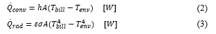

In (2)-(3),  [m²] represents the area related to the exposed surface,  [W/(m² K)] is the convection heat transfer coefficient,  [K] is the billet temperature and  [K] is the environment temperature of the fluid around the billet.  is the Stefan-Boltzmann constant and  is the emissivity coefficient [17].

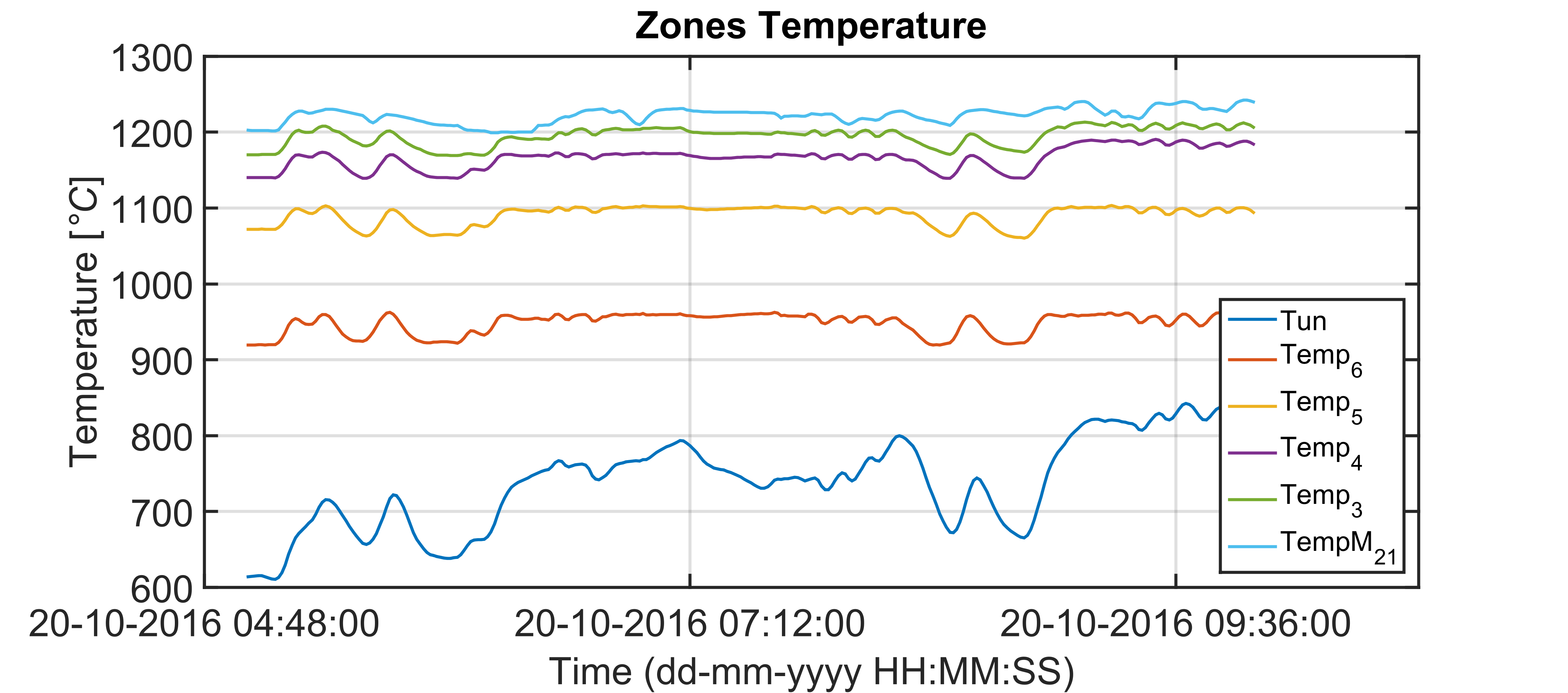
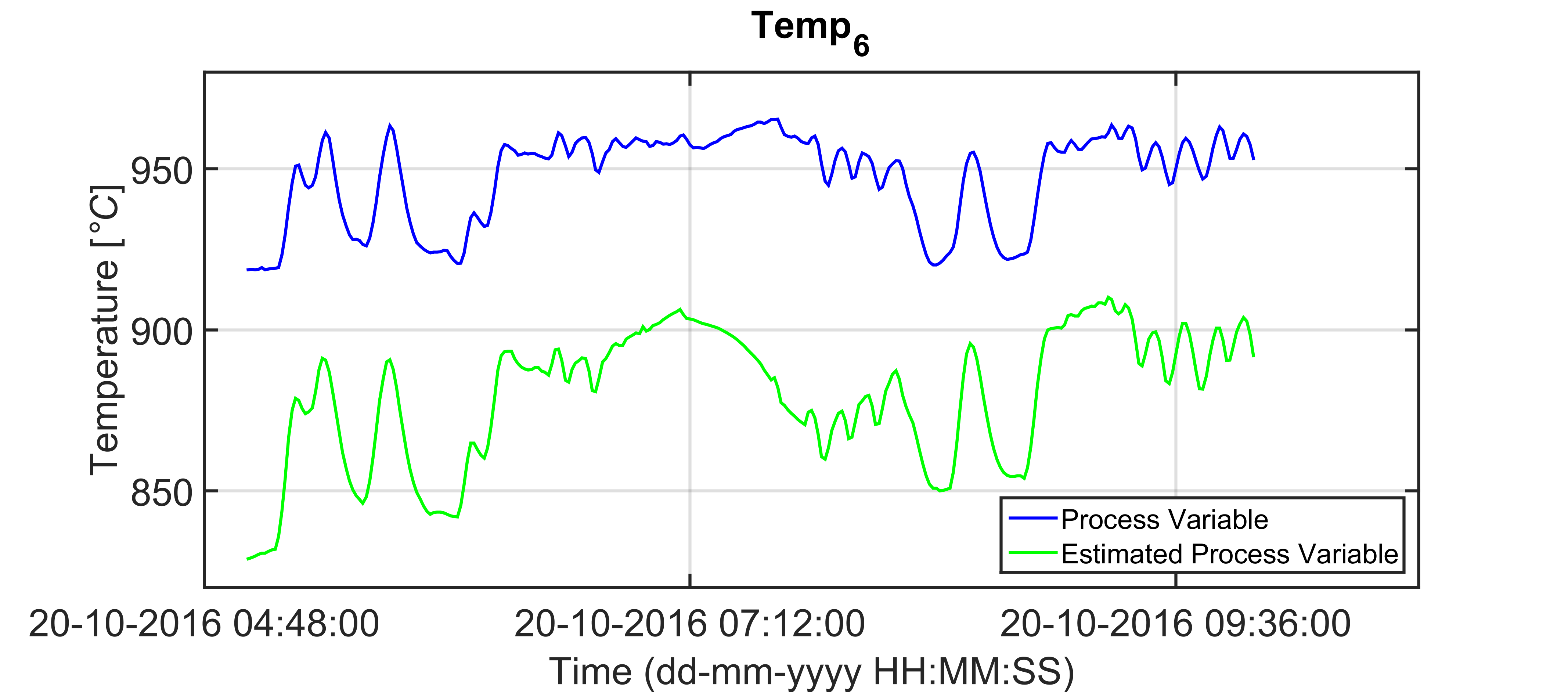
Through the equations reported in (1)-(3), a discretized model has been formulated for each billet that, at each considered sampling instant, lies in the reheating furnace. An important remark is the lack of an exact knowledge of the involved heat transfer coefficients. Online adaptation procedures for them have been included, based on customized constrained optimization problems that have been formulated exploiting feedback information. Figures 3-5 show an example of the virtual sensor field results related to October 2016. In Figure 3, blue stars indicate the measurements provided by the optical pyrometer in the rolling mill area; green stars represents the related virtual sensor temperature estimations. In Figures 4-5, trends related to the inputs of the virtual sensor model and related to the furnace production rate have been reported, respectively. Using the Root Mean Square Error of Prediction (RMSEP) as a performance indicator for the virtual sensor estimation, an RMSEP less than 10 [°C] has been detected (about 1 [%] of an optical pyrometer measurement range). In Figure 4, examples of zone temperatures ranges can be observed. Note the increasing monotonicity of the temperatures according to the proximity to the furnace outlet.

The virtual sensor nonlinear model has then been linearized, in order to include billets temperatures estimations within an MPC strategy based on linear models. A Linear Parameter-Varying (LPV) model has been obtained [18]. The billets temperatures have been included in an ad hoc group of Controlled Variables (CVs), denoted as bCVs (b) group. In the considered case study, the bCVs group is composed by 136 elements (m_b=136). All terms involved in the inputs vector related to the bCVs model, i.e. the temperatures of all furnace zones, have been included in an own group, called as zones Controlled Variables (zCVs, y) group. This group also includes temperature differences between adjacent furnace zones, smoke-exchanger temperature (T_SE, [°C]), and fuel valves opening position [12]. As typical in industrial APC applications, other two categories of measured input process variables have been defined: Manipulated Variables (MVs, u) and Disturbance Variables (DVs, d). The MVs group includes the six fuel flow rates (Fuel_i (i=1-6), [Nm³/h]) and the six stoichiometric ratios (R_i (i=1-6), []) related to  the furnace zones equipped with an own burners set. In DVs group,

Figure 3.   Virtual sensor results: rolling mill billets temperature.

Figure 4.   Virtual sensor results: inputs.

Figure 5.   Virtual sensor results: furnace production rate.

Figure 6.   Zone 6 temperature model performances.

the furnace production rate (Prod, [t/h]), the furnace pressure (FurnPress, [mmH2O]) and the air pressure (FurnPress, [mbar]) have been included. The zCVs-MVs/DVs relationships have been modelled through asymptotically stable linear time invariant models without delays on the input-output channels. Steady-state gain signs related to some zCVs-MVs/DVs models have been reported in Tables 3-4. The empty boxes indicate the absence of a relationship.

Figure 7.   Zone 5 temperature model performances.

Table 3: zCVs-MVs models: steady-state gains signs

Acronym	Fuel6	Fuel5	Fuel4	Fuel3	Fuel2	Fuel1
Tun	+	+	+	+	+	+
Temp6	+	+	+	+	+	+
Temp5		+	+	+	+	+
Temp4			+	+	+	+
Temp3				+	+	+
Temp2					+	+
Temp1					+	+
TSE	+	+	+	+	+	+

Table 4: zCVs-DVs models: steady-state gains signs

Acronym	FurnPress	Prod	AirPress
Tun	+	–	–
Temp6	+	–	–
Temp5	+	–	–
Temp4	+	–	–
Temp3	+	–	–
Temp2	+	–	–
Temp1	+	–	–
TSE	+	–	–

Note, in Table 3, that the temperatures of the furnace zones located closer to the furnace inlet are influenced by the fuel flow rates of the downstream zones. Figures 6-7 report examples of the performances of the models related to zone 6 and zone 5 temperatures. Green lines represent the model prediction while blue lines represent the field process variables. The depicted trends refer to the same period taken into account in the scenario proposed in Figures 3-5.

3. “i.Process | Steel – RHF” APC system

In this section, “i.Process | Steel – RHF” APC system technology is described, focusing on the optimization problems solved by the two MPC modules and on tuning procedures.

3.1.  APC Architecture Description

Figure 8 schematically describes “i.Process | Steel – RHF” APC system architecture. At each control instant k, a Supervisory Control and Data Acquisition (SCADA) system provides updated data; note the location of the developed billets temperature estimation virtual sensor. A Data Conditioning & Decoupling Selector (DC&DS) block receives updated process variables values (Figure 8, right side, u(k-1), d(k), y(k), b(k)). Furthermore, DC&DS block exploits other information, i.e. local control loops conditions (Figure 8, Plant Signals & Parameters), status information related to the selected process variables (Figure 8, right side, u-d-y-b Status), and control requirements related to MVs manipulation (Figure 8, right side, Decoupling Matrix) [19,20]. The status information related to the selected process variables defines which process variables have to be included in the MPC problem at each control instant. The Decoupling Matrix defines which MVs have to be moved by MPC strategy for the satisfaction of the specifications related to the zCVs. Table 5 shows the initial Decoupling Matrix provided to DC&DS block. For example, considering the zone 6 temperature, this zCVs is tied to all fuel flow rates (see Table 3); for this reason, without any expedients, all fuel flow rates could be moved by MPC system for the satisfaction of the zone 6 temperature specifications. According to some additional specifications that have been defined for the considered case study, only zone 6 fuel flow rate should be moved for the cited zCV. With regard to this aspect, observe the second row of Table 5 (related to zone 6 temperature): the “0” value indicates the MVs to be inhibited for its control [20].

Figure 8.   “i.Process | Steel – RHF” architecture.

Table 5: zCVs-MVs models: initial decoupling matrix

Acronym	Fuel6	Fuel5	Fuel4	Fuel3	Fuel2	Fuel1
Tun	1	1	0	0	0	0
Temp6	1	0	0	0	0	0
Temp5	1	1	0	0	0	0
Temp4	1	1	1	0	0	0
Temp3	1	1	1	1	0	0
Temp2	1	1	1	1	1	0
Temp1	1	1	1	1	0	1
TSE	1	1	0	0	0	0

Based on the received information, DC&DS block performs different operations and checks, e.g. bad detection and data conditioning. From this phase, the possibly modified process variables values (Figure 8, left side, u(k-1), d(k), y(k), b(k)), the final status values for process variables (Figure 8, left side, u-d-y-b Status) and the final Decoupling Matrix (Figure 8, left side, Decoupling Matrix) resulted. The final Decoupling Matrix contains information about process variables final status values and about MVs action inhibition specifications [20].

MPC block, based on all the detailed parameters and information, computes the current optimal input to be applied to the plant (Figure 8, u(k)). MPC block has been based on a two-layer scheme formulated on linear models, constituted by an upper layer module called as Targets Optimizing and Constraints Softening (Figure 8, TOCS) and by a lower layer module called as Dynamic Optimizer (Figure 8, DO). A Predictions Calculator module cooperates with the two-layer scheme.

3.2.  Two-Layer MPC Scheme

The MPC scheme exploits process variables predictions on a prediction horizon . The zCVs and bCVs free response ([13]) is computed by Predictions Calculator module (Figure 8, y Free Response and y-b Free Response).

At the upper layer of the proposed MPC scheme, TOCS module solves a Linear Programming (LP) problem. A linear cost function is minimized, subject to linear constraints: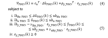

In the LP problem represented by (4)-(5), minimization or maximization directions for MVs can be preferred through  term that multiplies the MVs steady-state move .  is constrained by  and ; with regard to MVs, the steady-state value  is constrained by  and . zCVs steady state value  is constrained by  and . TOCS MVs constraints have been considered as hard constraints: they can never be violated and their feasibility has been suitably imposed. On the other hand, TOCS zCVs constraints have been considered as soft constraints: they can be violated thanks to the slack variables contained in  term. This term contains two nonnegative slack variables for each zCV; it has been introduced in (4) through  term and in (5) through  and  terms.

 In Figure 8, , , ,  are among u-y Constraints. ,   ,   and  terms are among TOCS Tuning Parameters.

TOCS module formulation exploits zCVs-MVs/DVs models and predictions at the end of the prediction horizon . Solving its LP problem, TOCS module computes MVs and CVs steady-state
targets (Figure 8, u- y Target) and zCVs constraints (Figure 8, y Constraints); these terms are provided to DO module [19,20].

At the lower layer of the proposed MPC scheme, DO module computes the  (  is denoted as control horizon [13]) optimal MVs moves, solving a Quadratic Programming (QP) problem. These moves are included in a  vector ( ).  represent the MVs movement instant ( ; ) [12]. A quadratic cost function is minimized, subject to linear constraints:

In the QP problem represented by (6)-(7), tracking errors over  between MVs and zCVs reference trajectories (  and ) and the related predicted values (  and ) are weighted by  and  positive semidefinite matrices.  and  are constrained by , ,  and . DO MVs moves are weighted in (6) by positive definite matrices  and they are constrained in (7) by  and . DO MVs constraints have been considered as hard constraints: they can never be violated and their feasibility has been suitably imposed. On the other hand, DO zCVs constraints have been considered as soft constraints: they can be violated thanks to the slack variables contained in  term. This term contains a nonnegative slack variable for each zCV; it has been introduced in (6) through  term and in (7) through  and  terms.

In Figure 8, , , ,  are among u-b Constraints.  and  terms are among y Constraints.  , , , ,  and  terms are among DO Tuning Parameters.

Taking into account the just described terms related to MVs and zCVs, and exploiting zCVs-MVs/DVs models, a first “i.Process | Steel – RHF” APC system control mode has been formulated, denoted zones APC mode.

Including terms related to bCVs in the DO QP problem represented by (6)-(7), a second control mode for “i.Process | Steel – RHF” APC system has been obtained, denoted adaptive APC mode. It constitutes the main control mode and it exploits, besides zCVs-MVs/DVs models, also first principles bCVs LPV model and billets virtual sensor information. In this way, an adaptive two-layer MPC strategy has been formulated. In (6)-(7), for the generic billet  that lies on the  ( )  furnace  place  at the current

control instant , its predicted furnace discharge instant is
computed ( ) taking into account the furnace production rate. The billets temperature predictions ( ) at the related furnace discharge instants  ( ) are constrained in (7) by  and  (Figure 8, u-b Constraints). These constraints have been considered as soft constraints: they can be violated thanks to the slack variables contained in  term. This term contains a nonnegative slack variable for each bCV; it has been introduced in (6) through  term and in (7) through  and  terms (Figure 8, DO Tuning Parameters). Tracking option of desired values ( ) for bCVs has been included in DO cost function (6), exploiting  nonnegative scalars.

3.3.  Tuning Details

Tailored tuning methods have been developed for optimizing the controller performances in the two defined control modes. The control moves are computed by the APC system once a minute, according to the formulated process model.

With regard to the choice of the prediction horizon , it varies based on the control mode that has to be exploited. Consequently, also the control horizon  and the MVs movement instants  are adapted. For example, in the simulation example that will be proposed in Section 4, the adaptive APC mode will be activated. In this case, a furnace movement time equal to about 95 [s] is assumed, which corresponds, for the present case study, to a furnace production rate equal to about 85 [t/h]. Accordingly, in order to guarantee the predicted reaching of the furnace outlet to the billet closer to the furnace inlet, a prediction horizon  of 216 [min] is set. In a parametric way, the control horizon  is set equal to 44 moves suitably spaced over the prediction horizon .

In TOCS module formulation, the elements of  have been set as positive, in order to prefer, within the process variables defined constraints, minimization directions for fuel flow rates and stoichiometric ratios. Furthermore, ,  and  terms have been set in order to guarantee the desired priority on constraints satisfaction. For example, constraints related to smoke-exchanger temperature are more important than those related to zones temperature: the related   ,   and  terms have been set accordingly to this specification, taking into account also the magnitude of the involved process variables.

In DO module formulation, common tuning aspects between the two formulated control modes have been proposed. The priority of the soft constraints terms (if these constraints are included in the controller setup) ,  and  is guaranteed; furthermore, zCVs constraints are always present within DO module formulation. The option of tracking desired reference trajectories related to MVs is another similar tuning aspect, together with the need to take into account the magnitude of MVs moves. In DO module formulation related to the adaptive APC mode, billets (tracking and/or constraints satisfaction) specifications can be considered; optimal trade-offs between control and energy efficiency specifications must be ensured.

4. Simulation Results

This section proposes some simulation results related to “i.Process | Steel – RHF” APC system. In particular, a simulation scenario where the adaptive APC mode is activated is described.

4.1.  A Simulated Scenario

The adaptive APC mode performances are shown through a
simulated scenario: the zCVs-MVs/DVs plant model exploits the identified zCVs-MVs/DVs model and no measurement noise is assumed. The plant model for simulating the relationships between billets temperature and furnace zones temperature is based on the developed billets temperature nonlinear model that is exploited by the virtual sensor.

At the initial control instant of the proposed simulation, the adaptive APC mode is requested to be activated. The virtual sensor estimation gives reliable results and bCVs (billets temperature) can be included in the control problem. The zCVs reported in Table 1, the temperature differences between the bCVs model inputs and all fuel flow rates represent the other process variables that are considered in the simulation. The other MVs and all DVs are considered constant, so not influencing the proposed simulation scenario. Constraints related to zCVs and fuel flow rates have been reported in Tables 6-7. The temperature differences between the bCVs model inputs are constrained so as to ensure an increasing monotonicity of the temperatures along the furnace. As mentioned in Subsection 3.3, the furnace production rate is equal to about 85 [t/h]; the temperature of the 136 billets that initially lie within the furnace is in the range 20 [°C] – 1140 [°C], while the billets that will enter the furnace during the simulation are characterized by a temperature of about 550 [°C]. The Rolling Phase specifications
Table 6: Simulation scenario: zCVs constraints

Acronym	Upper Constraint	Lower Constraint
Tun	950 [°C]	550 [°C]
Temp6	1150 [°C]	800 [°C]
Temp5	1150 [°C]	800 [°C]
Temp4	1200 [°C]	800 [°C]
Temp3	1250 [°C]	1000 [°C]
Temp2	1250 [°C]	1000 [°C]
Temp1	1250 [°C]	1000 [°C]

Table 7: Simulation scenario: MVs constraints

Acronym	Upper Constraint	Lower Constraint
Fuel6	800 [Nm3/h]	0 [Nm3/h]
Fuel5	1600 [Nm3/h]	0 [Nm3/h]
Fuel4	650 [Nm3/h]	0 [Nm3/h]
Fuel3	650 [Nm3/h]	0 [Nm3/h]
Fuel2	250 [Nm3/h]	0 [Nm3/h]
Fuel1	250 [Nm3/h]	0 [Nm3/h]

require that the billets temperature in the rolling area must be in the range 1030 [°C] – 1045 [°C]. This specification can be converted in a temperature range of about 1051 [°C] – 1066 [°C] at the furnace outlet. The “i.Process | Steel – RHF” adaptive APC mode ensures that the billets temperature detected by the optical pyrometer in the rolling mill area converges towards the minimum required temperature (1030 [°C]), as can be observed in Figure 9.

Figure 9.   Simulation results: bCVs trends.

Figure 10.   Simulation results: bCVs model inputs trends.

Figure 11.   Simulation results: Fuel6 trends.

Figure 12.   Simulation results: Fuel5 trends.

Figure 13.   Simulation results: Fuel4 trends.

Figure 14.   Simulation results: Fuel3 trends.

Figure 15.   Simulation results: Fuel2 trends.

Figure 16.   Simulation results: Fuel1 trends.

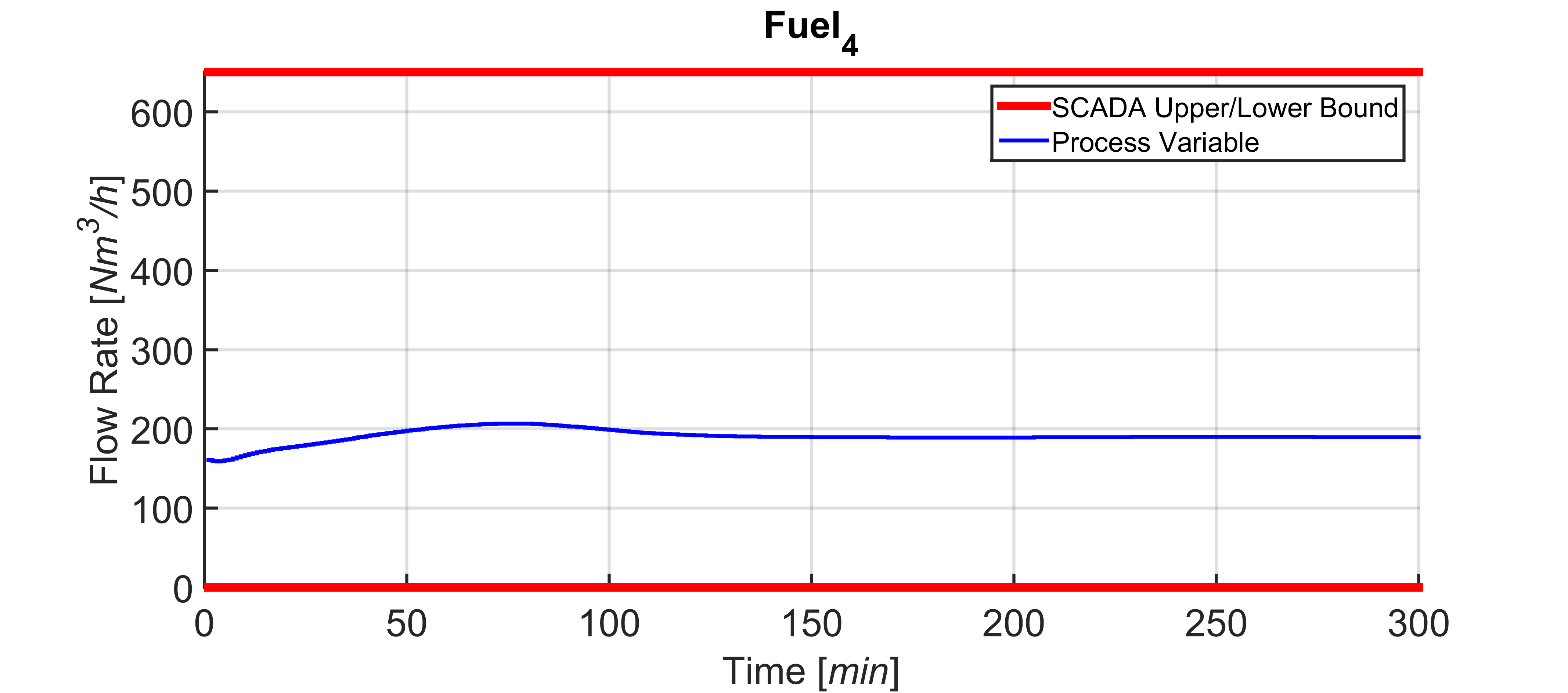
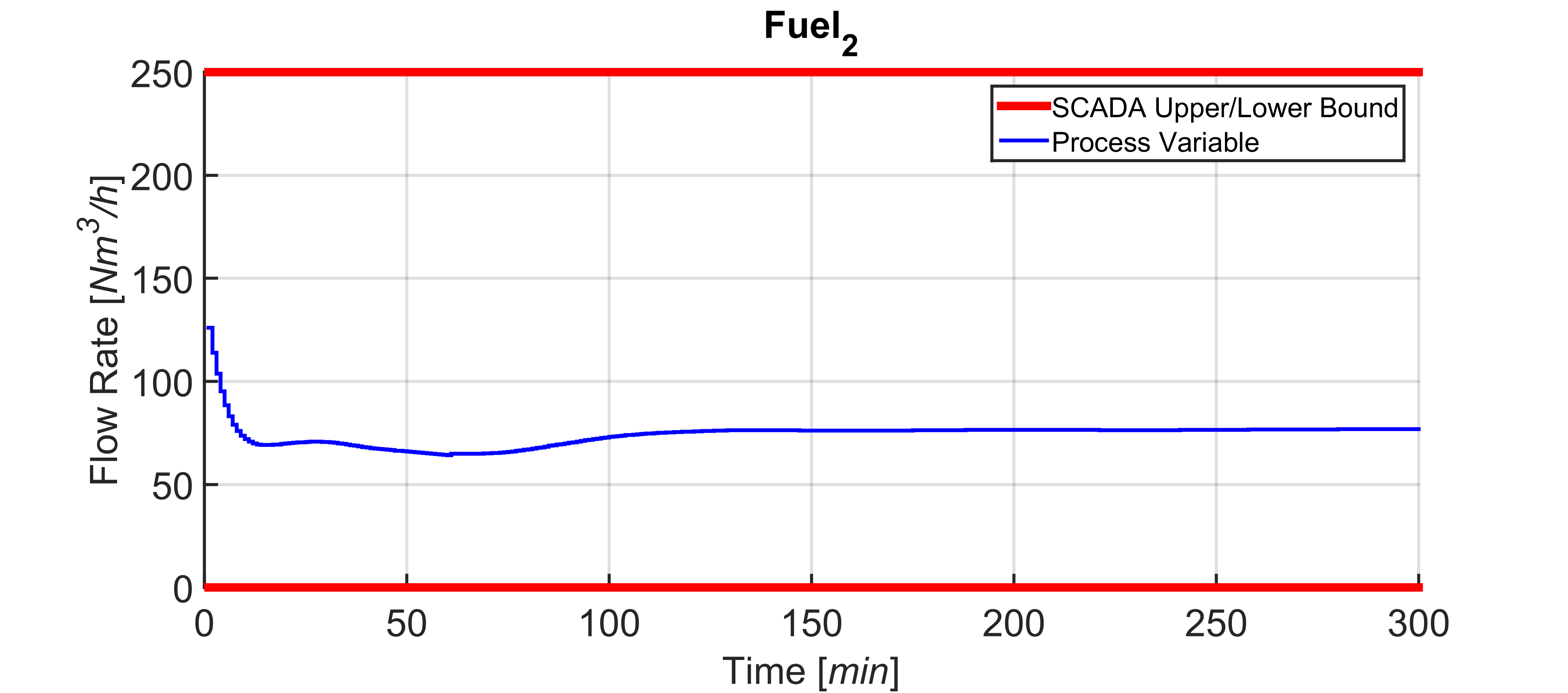
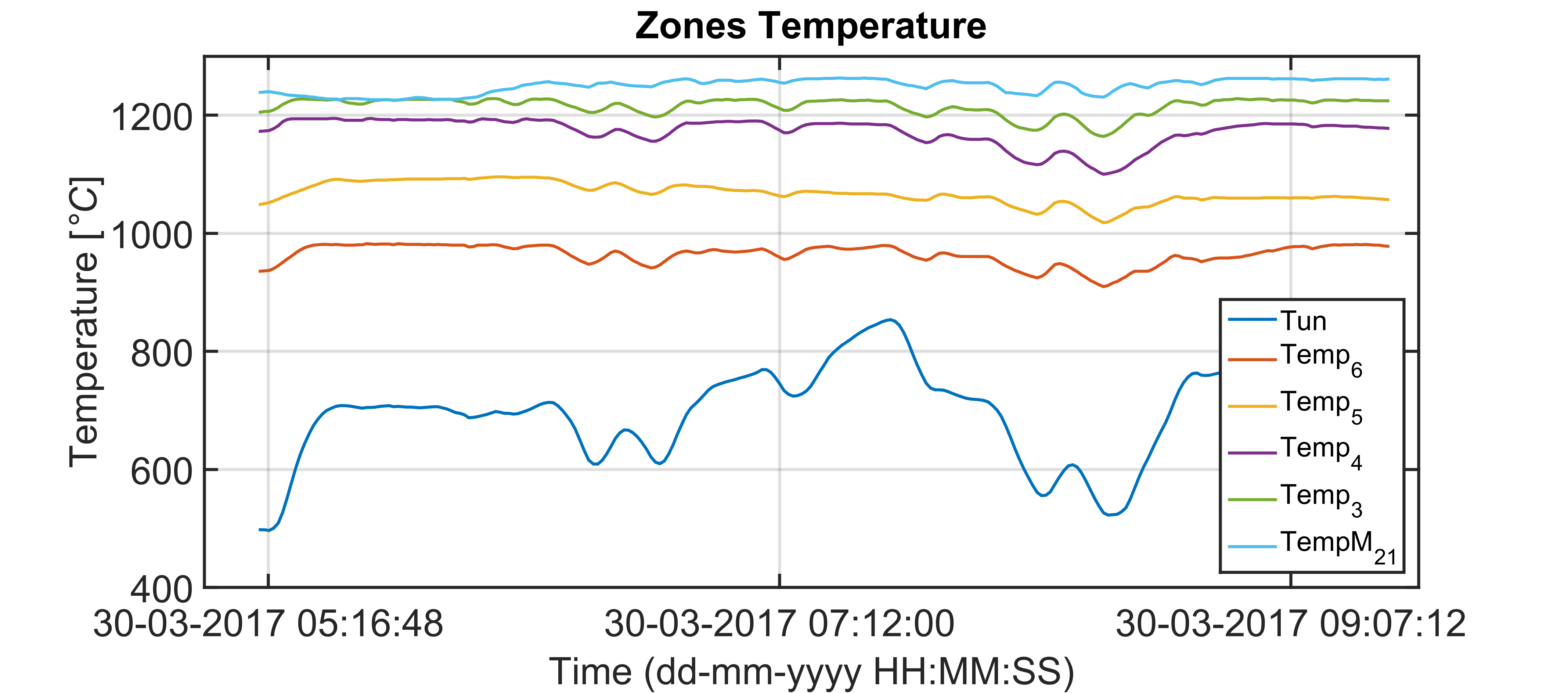
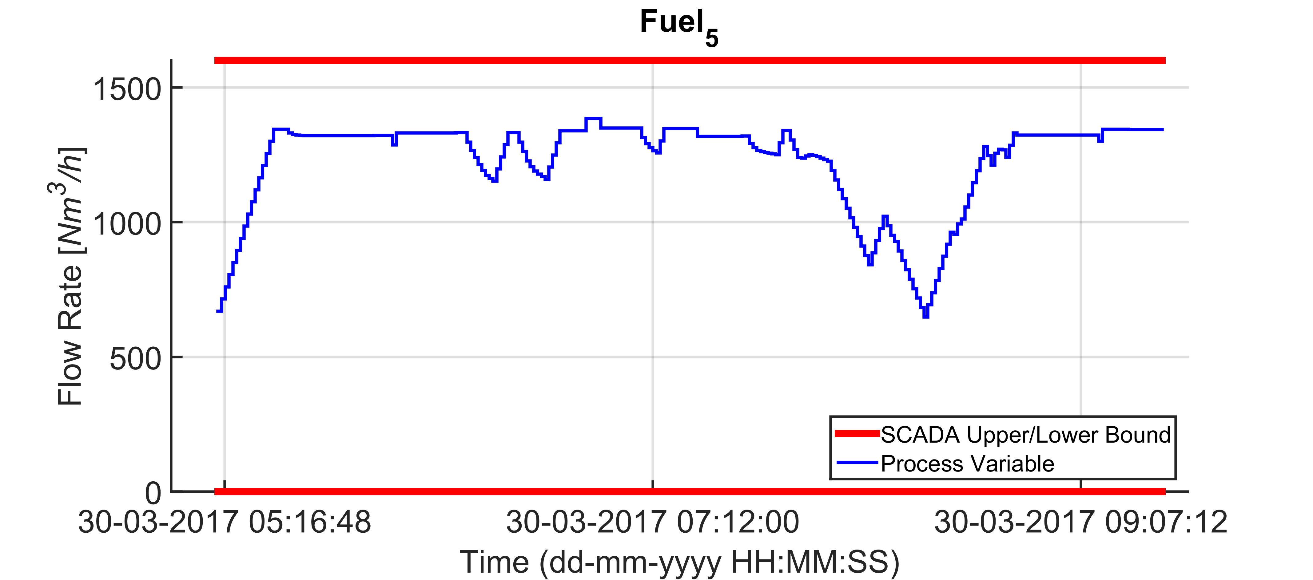
The cooperative action between TOCS and DO modules, that exploits virtual sensor information and billets temperature LPV model ensures a coordinated management of the furnace zones temperature (Figure 10) that is directly tied to the manipulation of the fuel flow rates (Figures 11-16). Consequently, a more profitable plant configuration is guaranteed that, at the same time, respect all the defined specifications. For example, in Figure 10, note the increasing monotonicity of the temperatures along the furnace.

5. Field Results

The study and design phases of the project related to the considered process began in January 2015 and ended in May 2015. The APC system has been installed on the considered Italian steel plant in early June 2015, substituting the local PID temperature controllers managed by plant operators. This section shows a plant scenario under the control of  “i.Process | Steel – RHF” APC system and some results about the obtained fuel specific consumption.

5.1.  A Plant Scenario

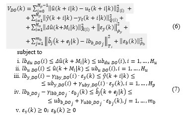
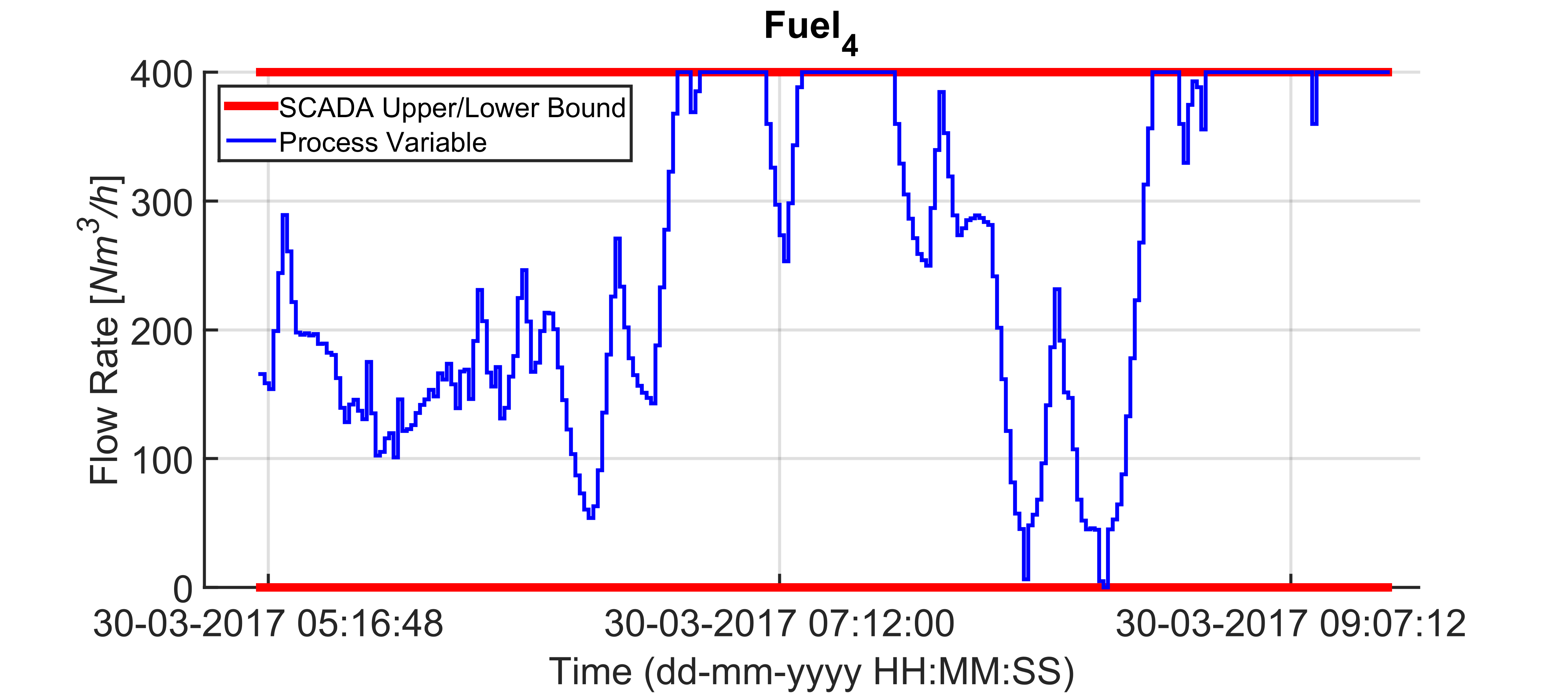
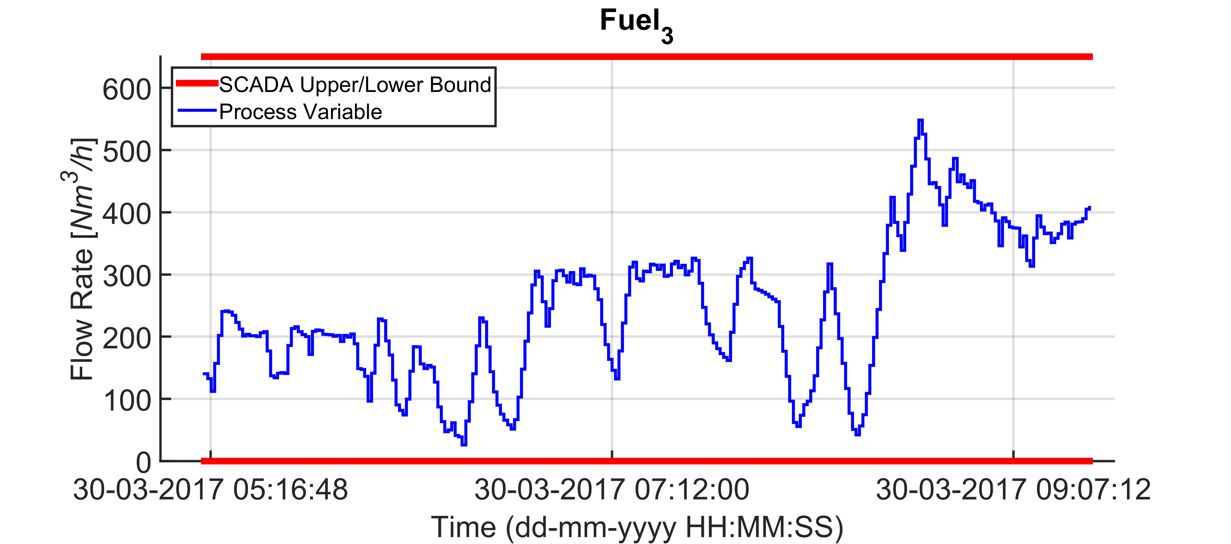
Figures 17-26 show a field scenario where “i.Process | Steel – RHF” APC system is active. A four hours period is taken into account. Figure 17 shows the bCVs trends: virtual sensor estimation and optical pyrometer measurements are depicted, together with the defined constraints in the rolling mill area (1125 [°C] – 1065 [°C]). The furnace production rate is shown in Figure 18, while the billets furnace inlet temperature is shown in Figure 19. The inputs related to the bCVs model are depicted in Figure 20 and Figures 21-26 show the fuel flow rates. Note the fuel flow rates trends (Figures 21-26, blue line) and the defined constraints (Figures 21-26, red lines). All MVs and DVs are considered in the control problem, together with some zCVs (furnace zones temperatures, temperature differences between adjacent furnace zones, smoke-exchanger temperature) and the bCVs (some process variables have not been shown for brevity). Examples of the constraints defined for the furnace zones and smoke-exchanger temperatures have been reported in Table 8. The 136 billets that are already present in the furnace at the beginning of the considered plant scenario are characterized by temperatures in the range 55 [°C] – 1100 [°C] and the inlet temperature of the billets that will enter the furnace is in the range 40 [°C] – 105 [°C] (Figure 19). Besides the inlet temperature of the billets, also the furnace production rate is not constant (Figure 18): it assumes a

Figure 17.   Field results: bCVs trends.

Figure 18.   Field results: furnace production rate trends.

Figure 19.   Field results: billets furnace inlet temperatures trends.

Figure 20.   Field results: bCVs model inputs trends.

Figure 21.   Field results: Fuel6 trends.

Figure 22.   Field results: Fuel5 trends.

maximum value that is equal to about 120 [t/h]. The furnace pressure and the air pressure (DVs) are about 0.9 [mmH2O] and 84 [mbar], respectively.

As can be observed in Figure 17, “i.Process | Steel – RHF” APC system ensures that the billets temperature detected by the optical pyrometer in the rolling mill area converges towards the minimum required temperature (1065 [°C]). The TOCS–DO cooperative action, exploiting virtual sensor information and billets temperature LPV model, ensures a profitable management

Figure 23.   Field results: Fuel4 trends.

Figure 24.   Field results: Fuel3 trends.

Figure 25.   Field results: Fuel2 trends.

Figure 26.   Field results: Fuel1 trends.

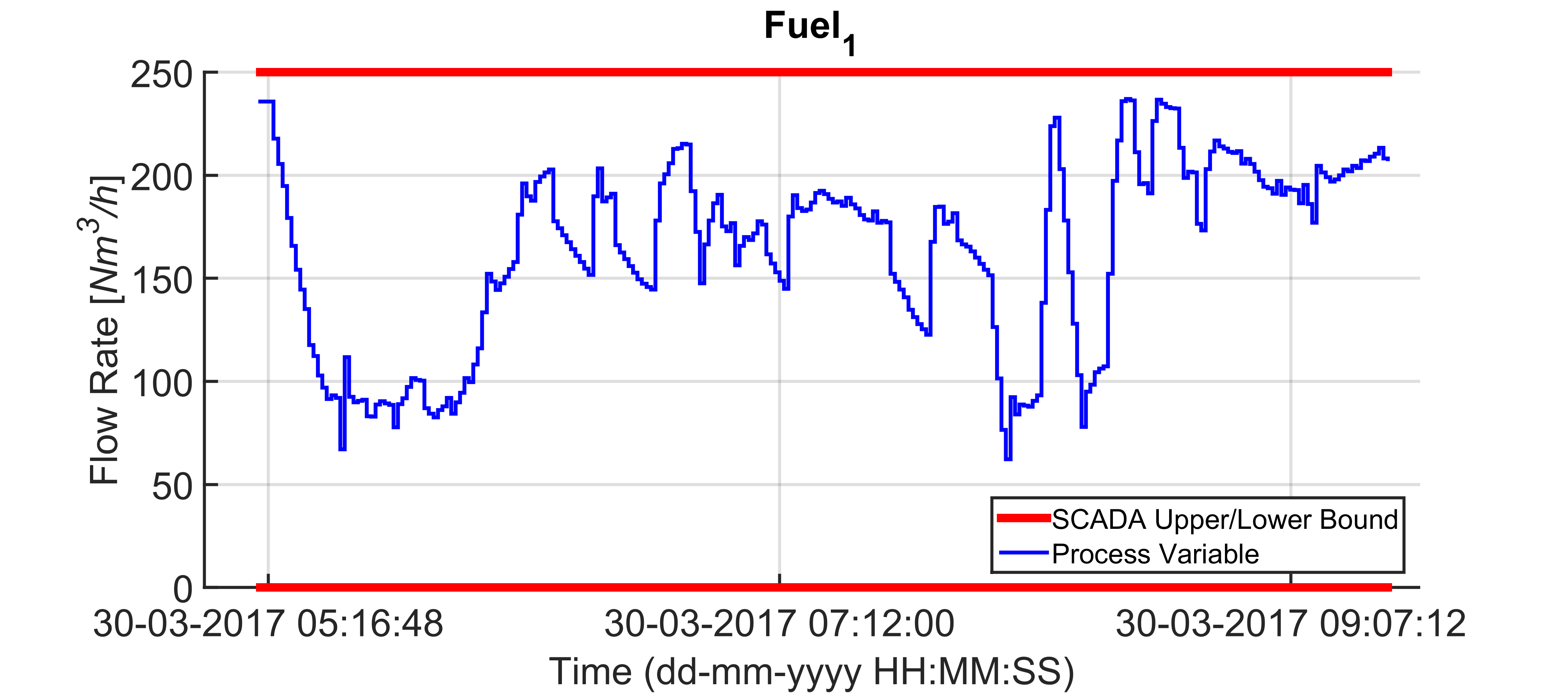
of the furnace zones temperature (Figure 20) that is directly tied to the manipulation of the fuel flow rates (Figures 21-26). All the imposed constraints and specifications are fulfilled, despite a not constant furnace production rate (Figure 18) and a not constant billets furnace inlet temperature (Figure 19). The benefits deriving from the proposed multivariable predictive approach led the controller to conduct the plant to very profitable operating regions, but, at the same time, all the control specifications are satisfied. As it will be shown in the next subsection, an energy efficiency

Table 8: Field scenario: zCVs constraints

Acronym	Upper Constraint	Lower Constraint
Tun	950 [°C]	400 [°C]
Temp6	980 [°C]	900 [°C]
Temp5	1100 [°C]	1050 [°C]
Temp4	1190 [°C]	1140 [°C]
Temp3	1220 [°C]	1190 [°C]
Temp2	1260 [°C]	1220 [°C]
Temp1	1260 [°C]	1220 [°C]
TSE	730 [°C]	300 [°C]

improvement has been obtained with the developed APC system, with respect to the previous furnace conduction.

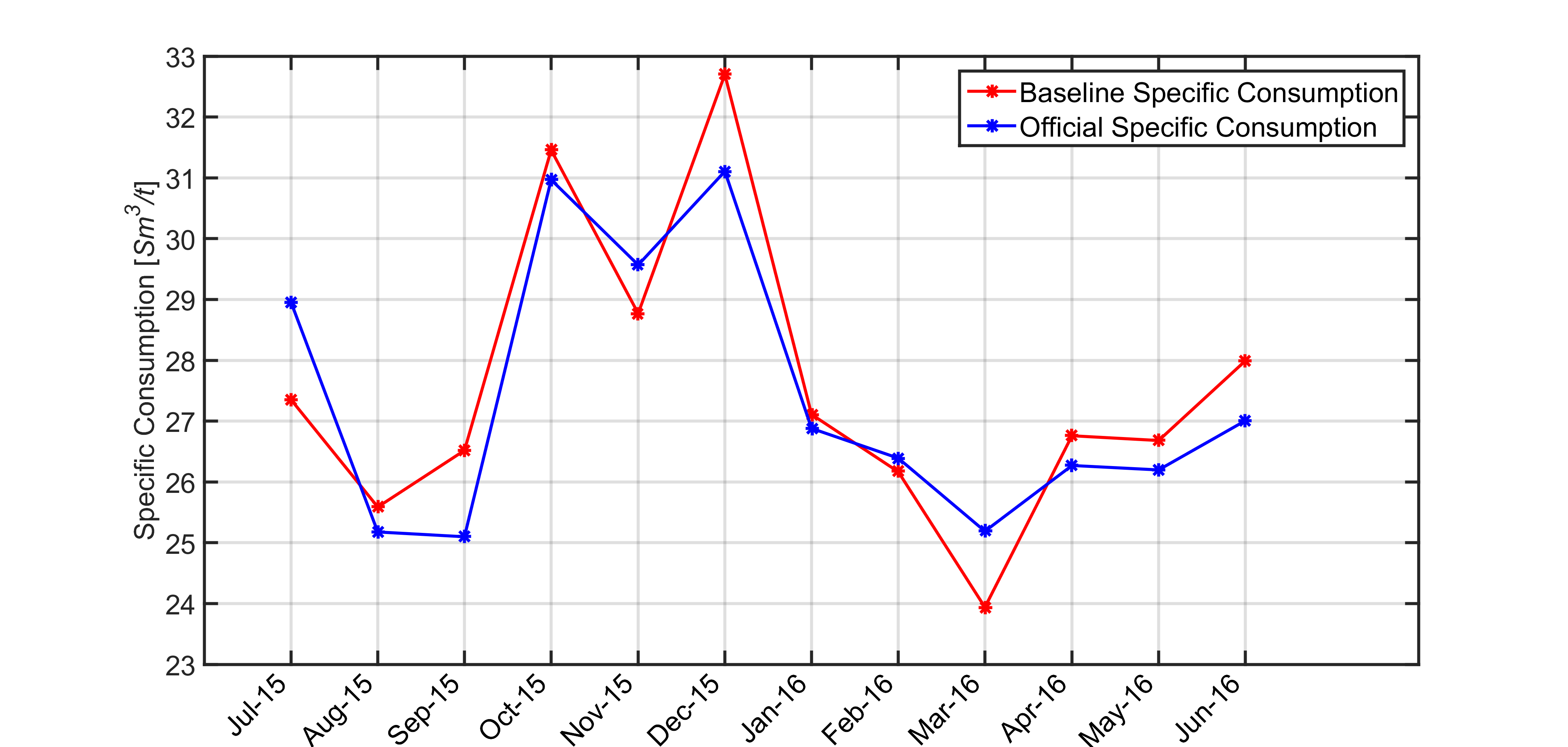
5.2.  Fuel Specific Consumption Results

The installation of the developed controller on the real industrial plant has guaranteed an improvement on the process control that has directly influenced the fuel specific consumption. The fuel specific consumption, that takes into account the fuel usage and the furnace production rate, represents a very significant indicator for the evaluation of the energy efficiency performances of “i.Process | Steel – RHF”. A project baseline for the fuel specific consumption has been computed, that varies with the furnace hot charge.

Figure 27 shows a subpart of a synoptic of the developed GUI: the daily fuel specific consumption ([Sm³/t]) is depicted. The “i.Process | Steel – RHF” APC system daily specific consumption

Figure 27.   Field results: comparison between daily baseline and daily official specific consumption.

Figure 28.   Field results: comparison between monthly baseline and monthly official specific consumption.

related to July 2017 is represented though a blue line, while the defined daily project baseline is shown through a red line. This page can be online monitored by plant operators; in this way, they can practically evaluate the controller performances from an energy efficiency point of view.

Figure 28 shows the monthly fuel specific consumption ([Sm³/t]) related to the first year of “i.Process | Steel – RHF” APC system performances. The specific consumption is represented though a blue line, while the defined project baseline is shown through a red line. After about two years from the installation of “i.Process | Steel – RHF” APC system on the described pusher type billets reheating furnace, about 2 [%] reduction of the fuel specific consumption with respect to the defined project baseline has been achieved. A controller service factor about equal to 95 [%] has been observed.

6. Conclusions

In this paper, an Advanced Process Control system aimed at optimizing a pusher type billets reheating furnace located in an Italian steel plant has been proposed. The control system, denoted “i.Process | Steel – RHF”, has been based on two-layer Model Predictive Control strategy formulated with linear models. The two-layer predictive controller also interacts with additional functional blocks.

Simulation and field results have demonstrated significant performances improvements guaranteed by the developed controller with respect to the previous control system based on Proportional Integral Derivative (PID) temperature controllers managed by plant operators. Thanks to the multivariable predictive approach, “i.Process | Steel – RHF” recognizes efficient operating zones and allows the process reaching them; in this way, process control and energy efficiency improvements have been guaranteed. Specifications related to the billets reheating are fulfilled and, at the same time, optimal configurations of the manipulated variables are reached. The developed control method has been patented [16].

After about two years from the installation of “i.Process | Steel – RHF” APC system on the described pusher type billets reheating furnace, about 2 [%] reduction of the fuel specific consumption with respect to the defined project baseline has been obtained, together with a controller service factor about equal to 95 [%].

1. enea.it
2. L. Latour, J. H. Sharpe, M. C. Delaney, “Estimating Benefits from Advanced Control” ISA Trans., 25(4), 13–21, 1986.
3. Bauer, I. K. Craig, “Economic assessment of advanced process control – A survey and framework” J. Proc. Contr., 18(1), 2–18, 2008. https://doi.org/10.1016/j.jprocont.2007.05.007
4. M. Canney, “Are you getting the full benefit from your advanced process control system?” Hydroc. Process., 84(6), 55–58, 2005.
5. Trinks, M. H. Mawhinney, R. A. Shannon, R. J. Reed, J. R. Garvey, Industrial Furnaces, John Wiley & Sons, 2004.
6. Martensson, “Energy efficiency improvement by measurement and control: a case study of reheating furnaces in the steel industry” in 14th National Industrial Energy Technology Conference, Houston Texas USA, 1992. http://hdl.handle.net/1969.1/92210
7. S. O. Santos, P. E. M. Almeida, R. T. N. Cardoso, “Fuel Costs Minimization on a Steel Billet Reheating Furnace Using Genetic Algorithms” Modelling and Simulation in Engineering, 2017, Article ID 2731902, 2017. https://doi.org/10.1155/2017/2731902
8. Yi, Z. Su, G. Li, Q. Yang, W. Zhang, “Development of a double model slab tracking control system for the continuous reheating furnace” International Journal of Heat and Mass Transfer, 113, 861–874, 2017. https://doi.org/10.1016/j.ijheatmasstransfer.2017.05.093
9. X. Liao, J. H. She, M. Wu, “Integrated Hybrid-PSO and Fuzzy-NN Decoupling Control for Temperature of Reheating Furnace” IEEE Trans. Ind. Electr., 56(7), 2704–2714, 2009. https://doi.org/10.1109/TIE.2009.2019753
10. Steinboeck, D. Wild, A. Kugi, “Nonlinear model predictive control of a continuous slab reheating furnace” Control Eng. Pract., 21(4), 495–508, 2013. https://doi.org/10.1016/j.conengprac.2012.11.012
11. Steinboeck, Model-based Control and Optimization of a Continuous Slab Reheating Furnace, Shaker Verlag GmbH, 2011.
12. Astolfi, L. Barboni, F. Cocchioni, C. Pepe, S. M. Zanoli, “Optimization of a pusher type reheating furnace: an adaptive Model Predictive Control approach” in 6th International Symposium on Advanced Control of Industrial Processes (AdCONIP), Taipei Taiwan, 2017. https://doi.org/10.1109/ADCONIP.2017.7983749
13. Maciejowski, Predictive Control with Constraints, Prentice-Hall, 2002.
14. F. Camacho, C. Bordons, Model Predictive Control, Springer-Verlag, 2007.
15. B. Rawlings, D. Q. Mayne, Model Predictive Control: Theory and Design, Nob Hill Publishing, 2013.
16. Astolfi, L. Barboni, F. Cocchioni, C. Pepe, “Metodo per il controllo di forni di riscaldo,” Italian Patent n. 0001424136 awarded by Ufficio Italiano Brevetti e Marchi (UIBM), 2016. http://www.uibm.gov.it/uibm/dati/ Avanzata.aspx?load=info_list_uno&id=2253683&table=Invention&
17. A. Cengel, Introduction to Thermodynamics and Heat Transfer, McGraw-Hill Companies, 2008.
18. Mohammadpour, C. W. Scherer, Control of Linear Parameter Varying Systems with Applications, Springer, 2012.
19. Pepe, “Model Predictive Control aimed at energy efficiency improvement in process industries,” Ph.D. Thesis, Università Politecnica delle Marche, 2017.
20. M. Zanoli, C. Pepe, “Two-Layer Linear MPC Approach Aimed at Walking Beam Billets Reheating Furnace Optimization” Journal of Control Science and Engineering, 2017, Article ID 5401616, 2017. https://doi.org/10.1155/2017/5401616

(Click to view)

(Click to view)