1. Introduction

The increasing demand of motorized vehicles is becoming one of the major problems that face the developed world places in nowadays. Based on some statistics in Great Britain, 90% of the journeys are by road, during the last decade, and for more the road distances travelled, have increased by over 1000% on the last sixty years. [1]

On-ramp metering [2] is being widely used as e method to increase the freeway operational efficiency by regulating the traffic interruption by minor roads, while maintaining the right of way on the major section until it reaches me critical densities, which assure the maximal flow [3]. Measure of the density on the major road is difficult to measure. In this paper is proposed a discretized traffic model (CTM) to obtain traffic densities which then will be accurate through Kalman Filter [4, 5 and 6].

2.  CTM model of a Highway with three cells

If we denote with ρ_i (k) the density of a cell (uniform or non-uniform length)_, instead of the number of vehicles n_i  on the a unit length cell, then we can bring equation (1.1)[6].

for density  of the cell i updated time step in (k+1), where T_s is the discrete time unit in seconds.

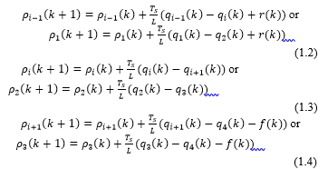
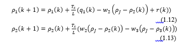
Analyzing a highway partitioned in three cells (for the sake of simply illustration)  with an on ramp and an off ramp, by assuming that the belonging cells can be in the free flow either in congested mode the densities on each cell can be written as in equations (1.2, 1.3, 1.4).

The densities on each cell are:

With the elaboration of the inter-cell flow law can be defined the expressions for the inter cell flows q₁, q₂ and q₃ in the above equations (1.1, 1.2 and 1.3). Before the inter cell flows elaboration is given, a reasonable description of the congestion must be given further, since as we assumed above, the cells can be in either free or congested mode. Congestion is defined as the state of the traffic with high density rates, or with other words the density of that part of the highway expressed in cell is equal or higher than the critical density based on the fundamental diagram of relationship of flow and density. Referred to the mentioned diagram, can be noticed that the congested flow belongs to higher values of the density, above the critical density values where the flow drops down. That can be described with enormous number of vehicles travelling at low speeds and with short distance spaces between each other.

The common modes, used in analysis of researchers are the fully congested mode when the three cells are congested, denoted by CCC mode, and free flow mode when the three cells are in free flow mode, denoted by FFF mode. The other middle modes that are out of the scope of this paper are those with last one and two cells in congested mode, written by FCC and FFC, respectively. To emphasize the modes, the congested cells are highlighted further.

Now, for the FFF mode, the densities of the cells are lower than the critical density and the inter cell flows are as follows:

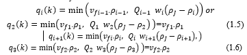
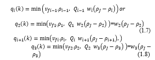
In CCC mode, the densities of the cells are higher that the critical density, and the inter cell flows are:

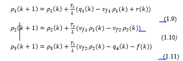
After subtracting the expressions for inter cell flows (1.5 and 1.6) in the equations of densities (1.2, 1.3 and 1.4), for the FFF mode, we have:

And after subtracting the expressions for inter cell flows (1.7 and 1.8) in the equations of densities (1.2, 1.3 and 1.4), for the CCC mode, we have:

3. State-Space presentation of CTM Model

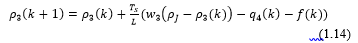
The state space presentation (particularly the state space, eq.1.17) of CTM based traffic densities of a highway segment in FFF mode differs from that of CCC mode. [7].

What it characterizes the state space model of the traffic density based on CTM model, is implication of some other extension parts of the state space, B_q which is the input matrix of upstream and downstream flows q₁ and q₄ respectively, B_r the input matrix for on ramp and off ramp flows, r and f respectively that are applicable on the FFF mode and input matrices, B_w which takes into consideration the backward waves w₂ and w₃ and B_J the input matrix of the jam density that are applicable on the state space model of the CCC mode. (1.17) and (1.18)

Where:   x (k+1) is the system state vector and in this paper, according to the CTM model, corresponds to the density in cell of cell i.

A is the state matrix, B is the input matrix, u(k) is the input or control and w_k   represents the process noise.

They are assumed to be independent (of each other), white, and with normal probability distributions (Gaussian) as: .

From the system of equations in (3.12, 3.13 and 3.14) can be drawn (after some regulations finding partial derivatives of the functions of densities to the parameters previous densities ρ(k),flows q₁ and q₄ and backward waves w₂ and w₃  which provide the elements of the respective matrices of the i^th row that correspond to density of i^th cell) the belonging matrices of the system matrices.

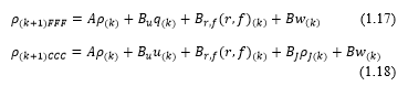
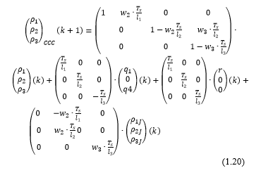
After bringing up together (eq. in 1.19 and 1.20 can be expanded to the form of state space: For FFF mode:

By recalling the standard state space models in (1.19) and (1.20), for completely free flow mode FFF and congested mode CCC respectively, there can be derived other variants, by changing the outflow from which is considered to have congestion the density formula, that is dictated by the backward speed and jam density of the downstream cell.

For CCC mode:

4. A numerical example of the CTM model-Traffic density

For the purpose of the demonstration of the CTM model, in this paper is performed a numerical example which is described below. For the sake of simplicity, are chosen the approximately the same freeway segment partitioning characteristics as that in earlier sections in order to do an interconnection with the laid state space model of traffic density. The system of performance measurements of the   traffic road networks of the Californian state PeMs is used for traffic collection data and is considered a freeway link for on the street “Broadway Avenue”, Stockton/San Francisco. The freeway is consisted from three cells with different lengths with one on-ramp on the first cell. (fig.1).

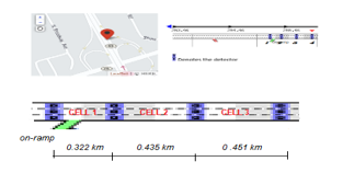Fig. 1. Freeway segment with three cells

Calibrated parameters are given below [8].

Table 1. Summary of traffic parameters for three cells
	QM	vf	ρcr	ρJ	w	FF/ /CC
Cell 1	5580	84.8	65.8	248	30.6	FF
Cell 2	4176	96.8	43.1	248	20.3	FF
Cell 3	4268	106.7	40.0	248	20.5	FF

The negative sign on the value q₄ denotes the flow exiting from last cell respectively flow exiting the highway segment while the positive q₁ characterizes its increasing sense of the density on the first cell.

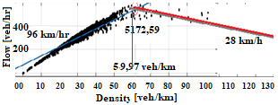Fig.2. Calibrated parameters

5. Kalman Filter

Kalman filter-KF (Kalman, 1960; Welch and Bishop 2001) is a recursive data processing algorithm that uses only the previous time-step’s prediction with the current measurement in order to make an estimate for the current state [4]. This means the KF does not require previous data to be stored or reprocessed with new measurements.

• The building structure of the KF

The Kalman Filter consists of a set of mathematical

equations that provides an efficient recursive computation to estimate the state of a process by minimizing the mean of the squared error. [4] The KF estimates the value of the variable x at any time (k+1), represented by a linear stochastic equation.

Where: A (k) is matrix which relates the state a time interval k with the state at current time interval k+1. B (k) is matrix which relates the current state to the control input .

The random variable w represents noise in modelling process. It is assumed to be within normal probability distributions with zero mean and variance Q (Gaussian) as:

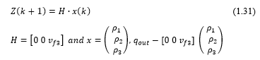
The system measurement equation describes the relationship between system states and measurements. Acknowledging that measurements inevitably contain noise, the output equation is expressed as follows:

 is the measurement variable (outflow of vehicles from cell 3-measured by loop detector 2) H (k) is the output matrix, and v (k) is the measurement noise variable. The errors in estimating a priori and a posteriori states are defined as follows:

The a priori and a posteriori estimate covariance is given by:

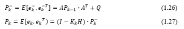The KF estimates a posteriori state of the process using a linear combination of a priori state and a weighted difference between the actual measurement and the model measurement of the state.

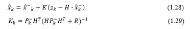Based on the above equation, especially on (1.29), the KF process can be divided in two steps ore phases. The first step is the prediction step and the second step is the correction step.

6. Estimation with Kalman Filter

              In this section are described in detail the applied matrices to the algorithm of the CTM-KF model. It is necessary to recall the equations state space of CTM model (Section V.1) first and then to do an interconnection of it with the KF algorithm equations. Since in our model, we are estimating the traffic densities of the three cells of the mentioned link, by the usage of the inputs values of the inflow q₁, output values q₄ and the flow from on ramp, then the state space vector of our algorithm are the densities x=[x₁,x₂,x₃]= [ρ₁, ρ₂, ρ₃]^T ,the input  vectors are

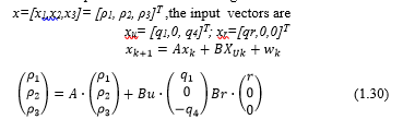
On this paper we are going to use the measurement of the outflow from the cell three, that corresponds to the flow q₄ in the figure (3.1). Based on the fundamental diagram we model the traffic flow measurement through the densities on the last cell (  and the free flow speed on cell 3 v_f3 we will have  that is consistent with the equation (6.2)

Where: Q -the model error covariance matrix which elements standard deviations of the density variables. The off diagonal elements are equal to zero while R is the measurement or output error covariance. In this seminar paper, the matrices Q and R are assumed to be constant.[9]

7. Results and Conclusion

Evaluation of the density values of cell is performed with discrete time intervals of T_s=10 seconds, where the initial values of the densities ρ₀ = [ρ₁₀, ρ₂₀, ρ₃₀ ]^T and estimated covariance matrix P_o are assumed. T_s is chosen to be 10 second in order to fill the conditions T<L/v _f , for proper work with system matrices, otherwise there will be obtained negative values of density parameters. For the purpose of the results evaluation, measured traffic densities for five minute intervals are used for comparison with the estimated densities with CTM model. The performance of the model was quantified by calculating the Mean Absolute Percentage Error (MAPE) given in (1.32).

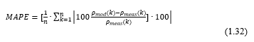The MAPE results for CTM model for modes FFF -KF,

for Cell 1, Cell 2 and Cell3, 2 %, 0.6 % and 1 % respectively,  nd for CCC-KF, 14% on the three cells. The results of the estimated values by CTM model against the measured values of traffic density are also graphically  presented on the below figure (3-5).

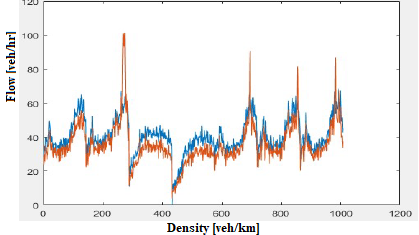Fig.3. Graphic results densities of KF FFF and measurements-

Cell 1

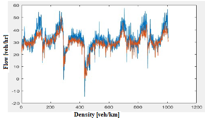Fig.4. Graphic results densities of KF FFF and measurements-

Cell 2

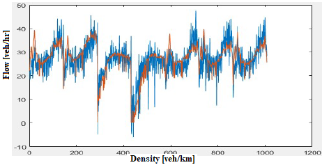Fig.5. Graphic results densities of KF FFF and measurements- Cell3

1. Nicola George – Kathryn Kershaw, Road Use Statistics, Great Britain, 2016
2. Ramp Metering: A Review of the Literature, E.D. Arnold ,Jr (1998)
3. Chen X.M, Li, L; Stochastic Evolutions of Dynamic Traffic Flow Modeling and Applications, Chapter 2, http://www.springer.com/978-3-662-44571-6 Springer (2015)
4. J .Lighthill ; G.B. Whitham “On Kinematic Waves, II: A theory of traffic flow on long crowded roads, Proceedings of the Royal Society of London, Series A-Mathematical and Physical Science.
5. Sun, L. Munoz. R. Horowitz, A Mixture Kalman Filter Highway Congestion Mode and Vehicle Density Estimator and its Application (2004)
6. Carlos F. Daganzo, “The Cell Transmission Model: Network Traffic”, (1996)
7. Munoz, X. Sun, R. Horowitz, L. Alvarez; “Traffic Density Estimation with the Cell Transmission Model1” (2003)
8. B. Witham “Linear and Nonlinear Waves”, Pure and Applied Mathematics, John Wiley Sons, New York City, USA, (1974)
9. Munoz, X. Sun, R. Horowitz, D. Sun, G. Gomes; “Methodological calibration of the cell transmission model” Proceedings of the American Control Conference, Massachusetts 2004.
10. Katsivalis, M. Papa Georgiou, ‘The importance of Traffic Flow Modeling for Motorway Traffic Control’, 2001

(Click to view)

(Click to view)