1. Introduction
Vowel classification has been an attractive research field with growing intensity over the recent years. It is closely related to voice activity detection, speech recognition, and speaker identification. Vowels are the main parts of speech and the basic building units of all languages and an intelligible speech would not be possible without them. They are the high energy parts of speech and also show almost periodic patterns. Therefore, they can be easily identified by time characteristics of their speech waveforms. Each vowel is produced as a result of vocal cord vibrations. The frequency of these vibrations is known as pitch frequency, which is a characteristic feature of the speech and the speaker. Pitch frequency variations occur mainly at voiced parts which are mostly formed by vowels. Consequently, vowels are an important source for features in speech processing.
Detecting the locations of the vowels in an utterance is critical in speech recognition because their order, representing the syllable form of the word, can help in determining the possible candidate words in speech. In addition, voice activity detection can be accomplished by determining the voiced parts of the speech which are mainly constituted from vowels. Speech processing technologies using spectral methods are also dependent on vowels and other voiced parts in speech. These methods are mostly built on the magnitude spectrum representation, which displays peaks and troughs along the frequency axis. Voiced segments of speech cause such peaks in the magnitude spectrum. The frequencies corresponding to the peaks, known as formants, are useful for both classifying the speech signal and identifying the speaker. Therefore, vowels are inevitable in the area of speech processing [1].
There are quite a number of studies on vowel classification in the literature. Most of them are based on frequency domain analysis using features such as formant frequencies [2,3], linear predictive coding coefficients (LPCC), perceptual linear prediction (PLP) coefficients [4], mel frequency cepstral coefficients (MFCC) [5,6,7,8], wavelets [9], spectro-temporal features [10], and spectral decomposition [11]. However, there are fewer studies using time domain analysis [12, 13]. There are also vowel classification studies for the imagined speech [14].
Although most of the studies on speech recognition make use of the acoustic features, the visual characteristics obtained from speech waveform shapes can also carry meaningful information to represent the speech. Shape characteristics, for example, envelope of the waveform, area under that waveform, and some other geometrical measurements can be utilized for classification purposes. Extracting these properties can be accomplished by basic image processing techniques such as edge detection and morphological processing. In other words, a speech waveform can be treated as an image. The notion of visual features is perceived as the shapes of the mouth and lips in general, and used also in vowel classification [15]. There exist some articles in the literature concerning the speech and sound signals as an image. Many of them utilize visual properties from the spectral domain. Matsui [16] et al. propose a musical feature extraction technique based on scale invariant feature transform (SIFT), which is one of the feature extractors used in image processing. Dennis et al. [17] use visual signatures from spectrogram for sound event classification. Schutte offers a parts-based model, employing graphical model based speech representation, which is applied to spectrogram image of the speech [18]. Dennis et al. [19] propose another method for recognizing overlapping sound events by using visual local features from the spectrogram of sounds and generalized Hough transform. Apart from these time-frequency approaches, Dulas deals with the speech signal in the time domain. He proposes an algorithm for digit recognition in Polish making use of the envelope pattern of the speech signal. A binary matrix is formed by placing a grid on the speech signal of one pitch period. Similarity coefficients are, then, calculated by comparing the previous and next five matrices around the matrix to be analyzed [20, 21]. Dulas also implements the same approach for finding the inter-phoneme transitions [22].
In this paper, we propose the visual features obtained from the shapes of speech waveforms to classify vowels. We are inspired by the fact that one can determine the differences among the vowels by visually inspecting their shapes. The proposed approach, called herein Speech Vision method (SV), henceforth considers the speech waveform as an image. The images corresponding to the respective vowels are formed from two-pitch period speech segments. After applying several image processing techniques to these waveform images, some useful geometrical descriptors are extracted from them. Later, these descriptors are used for training Artificial Neural Network (ANN), Support Vector Machine (SVM), and eXtreme Gradient Boosting (XGB) models to recognize the vowels. Experiments show that comparable recognition rates are obtained. The use of visual features makes a clear distinction between the application areas of classical frequency domain approach and our suggested method. A possibility of application is in the field of language education, especially language learning of a foreign language, where one needs to test learner’s pronunciation of vowels, or the learner tries to make the shape of the vowel as he/she sees both his/her own pronunciation and the ideal shape of the corresponding vowel on a screen for example. By the same token, the method could also be used in the speaking education of those with hearing disabilities. Another alternative area of application would be text to speech conversion tasks, in which ideal vowel shapes could be used in order to enhance the quality of the digital speech.
This paper is organized as follows. After this Introduction part, in Section II we discuss vowels and their properties. Section III presents the proposed method in details. Tests and results are given in Section IV, and a comparison with other vowel classification studies in the literature is carried out in Section V. Finally, conclusions and discussion appear in Section VI.
2. Characteristics of Vowels
In the Turkish language, there are 8 vowels and 21 consonants. The vowels are {a,e,ı,i,o,ö,u,ü}. There are 44 phonemes, 15 of which are obtained from vowels and the rest from consonants. The production of vowels basically depends on the position of the tongue, lips and jaw. For instance, for the vowel “a”, tongue is moved back, lips are unrounded and the jaw is wide open. Therefore, all the vowels are generated differently depending on the various positions of the parts of the mouth. By considering the shape of the mouth, Turkish vowels are distributed as given in Table 1 [23]. According to this table, there are several categories for the vowels. For example, {a,ı,o,u} are vocalized with the tongue pulled back, while {e,i,ö,ü} are vocalized with the tongue pushed forward. Similarly, {a,e,ı,i} are generated with lips unrounded and {o,ö,u,ü} are generated with lips rounded. We establish vowel groups to be classified in this study according to the position of lips and jaw.
Table 1: Classes of Turkish vowels
|
Unrounded (lips) |
Rounded (lips) |
| Wide (jaw) |
Narrow (jaw) |
Wide (jaw) |
Narrow (jaw) |
Back
(tongue) |
a |
ı |
o |
u |
Front
(tongue) |
e |
i |
ö |
ü |
When a voice plot is stated, it is basically meant to be the graph of voice intensity against time. A sample plot of a recorded vowel is given in Figure 1.
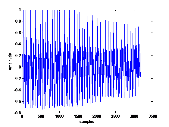 Figure 1: Waveform of Vowel “a”
It is noted that the vowel has a certain waveform. If we take a closer look, we can see that there is a repeating pattern in the waveform. This pattern is illustrated in Figure 2. The duration of each repeating pattern is known as the pitch period. This pattern keeps repeating with slight perturbations until the intensity starts to die off. When we focus on an interval of one pitch period of waveforms of all the vowels, we obtain the shapes illustrated in Figure 3. The vowels used in this paper come from a database [24]. As seen in that figure, each waveform generally differs from others in terms of appearance. The similar pattern can be experienced in certain English vowels, which sound like their corresponding Turkish counterparts. Figure 4 shows these vowels chosen from the words within parenthesis.
The argument in this study is that the vowels can be identified by examining their waveform shapes as an image. In other words, visual features extracted from the waveform images can make vowel classification possible without the need for spectral features such as MFCC, LPCC and/or PLP coefficients. From this point of view, the proposed technique contributes to the feature selection part in speech processing. Therefore, some of the image processing and machine vision techniques are applied to those waveforms. The main novelty of this work lies in providing visual features for speech waveforms.
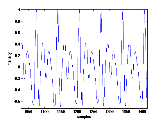 Figure 2: Repeating Patterns in Vowel “a”
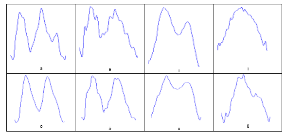 Figure 3: Sample Pitch Period Plots for 8 Turkish Vowels
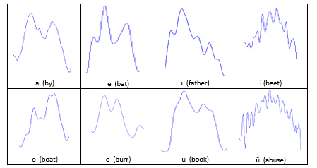 Figure 4: Sample Pitch Period Plots for 8 of the English Vowels
 Figure 5: Proposed Method for Vowel Classification
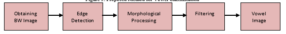 Figure 6: Operations in the “Visual Processing of ROI”
3. Speech Vision Methodology
The overall view of our proposed method is shown in Figure 5. In addition, Figure 6 shows the operations carried out in “Visual Processing of ROI” block. Our method comprises four main parts: the first is the extraction of Region of Interest (ROI), the second is visual processing of ROI, the third is extraction of shape features, and the fourth is the ANN/SVM/XGB part, where inputs are formed from the matrix and fed into the previously trained model to obtain a classification result. The following subsections explain the functions of each block in detail.
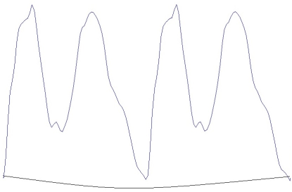 Figure 7: A Sample Closed Shape of Double Pitch Periods
3.1. Processing of region of interest
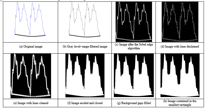 Figure 8: Steps for Image Operations
The input speech signals are segmented into two-pitch length waveform images as seen in Figure 7. The reason for choosing double pitch periods is that the shapes of a single, double, and triple pitch periods are compared, and two consecutive pitch periods give the highest scores in classification. As can be seen in Figure 8a, the image contains little jagged edges because of the noise level and the style of the speaker. In order to make vowel recognition speaker independent, one should dispose of those rapid ups and downs. Hence, we apply a sequence of image processing operations to smooth these details and, consequently, obtain a more general appearance of the waveform.
A selected waveform image to be processed is shown in Figure 8a. Then, a range filter which calculates the difference between maximum and minimum gray values in the 3×3 neighborhood of the pixel of interest is applied to the obtained gray-level image. The resulting image can be seen in Figure 8b. After this, we determine the edges of this image using Sobel algorithm with a threshold value of 0.5.
The image obtained is shown in Figure 8c. Following this, we apply a morphological structuring for line thickening, whose result is given in Figure 8d. Then, we clear the edges and borders using 4-connected neighborhood algorithm and obtain the image shown in Figure 8e. Following this operation, we erode the image and close it using a morphological closing method, whose result is shown in Figure 8f. Finally, the gaps on the background are flood-filled while changing connected background pixels (0’s) to foreground pixels (1’s). The result is seen in Figure 8g. A closing operation is applied to this figure and the resulting image is later contained in the smallest rectangle as depicted in Figure 8h. In the morphological operations performed on the images, we used structuring elements of line with length of 3 and angles of 0 and 90 degrees, as well as diamond with size of 1 and disk with size of 10.
3.2. Extraction of shape features
The geometric features that characterize the waveform image seen in Figure 8h are presented in this section. Since the aim is to analyze the rough shape rather than the detailed one, the features are selected in a way that represents the general silhouette of the waveform. The authors in [25] used ten features describing the general silhouettes of aircraft. In this study, we use these features along with the orientation angle as an additional feature. Table 2 lists these features. They are calculated by using the function of regionprops in Matlab [26]. In the features F1, F2, F6, and F11, the white region in Figure 8h, referred to as the image region, is approximated by an ellipse.
The followings are the descriptions of the features;
Table 2: Features Obtained from the Processed Image
| Feature |
Name of the feature |
| F1 |
Major axis length |
| F2 |
Minor axis length |
| F3 |
Horizontal length |
| F4 |
Vertical length |
| F5 |
Perimeter |
| F6 |
Eccentricity |
| F7 |
Mean |
| F8 |
Filled area |
| F9 |
Image area |
| F10 |
Background area |
| F11 |
Orientation angle |
F1- Major axis length: the length of the longer axis of the image region in pixels. See Figure 9.
F2- Minor axis length: the length of the shorter axis of the image region in pixels. See Figure 9.
F3- Horizontal length: horizontal length of the image region in pixels. See Figure 10.
F4- Vertical length: vertical length of the image region in pixels. See Figure 10.
F5- Perimeter: perimeter of the image region in pixels, shown in red. See Figure 10.
F6- Eccentricity: a parameter of an ellipse indicating its deviation from the circularity, whose value ranges from 0 (circle) to 1 (line).
F7- Mean: the ratio of the total number of 1’s in the binary image to the total number of pixels.
F8- Filled area: the total number of white pixels in the image.
F9- Image area: estimated area of the object in the image region which is correlated with the filled area. The area is calculated by placing and moving a 2×2 mask on an image. Depending on the corresponding pixel values in the mask, the area is computed. For example, if all the pixels in the mask are black, then the area is zero. When all are white, then the area equals one. The other distributions of pixels in the mask result in area values between zero and one.
F10- Background area: estimated area of the black region in the image.
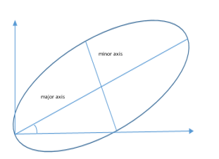 Figure 9: Major Axis, Minor Axis, and Orientation Angle
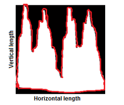 Figure 10: Horizontal and vertical lengths, and perimeter
F11- Orientation angle: the angle between the horizontal axis and the major axis of the ellipse approximating the image region. See Figure 10.
All the features describe the spatial domain properties of the underlying image. On the other hand, these images are the time domain representations of the speech signals. Thus, classifying the images corresponds to recognizing the speech sounds. Adopting such simple features in speech recognition leads to promising results, as shown in our experiments.
3.3. Classifiers
A general description of the employed classifiers is given here in order to facilitate a better understanding. We utilized three widely used classifiers in our study; namely ANN, SVM, and XGB method. It is well known that these are among the strongest classification tools for pattern recognition applications. They are all able to classify nonlinearly distributed input patterns into target classes. The classifiers are trained using the features in Table 2.
When sounding a vowel; the position of mouth, tongue, and lips is the key factor. The dotted and non-dotted (front and back) vowels in Turkish are quite similar in the way that only the position of the tongue changes when sounding the dotted and non-dotted vowels. Out of the eight vowels in Turkish, five vowel classes are formed in this study, combining ‘dotted’ vowels with non-dotted ones. Those combined vowels were: ‘ı’ and ‘i’, ‘o’ and ‘ö’, ‘u’ and ‘ü’. Besides, the vowels ‘a’ and ‘e’ are treated as separate classes. Therefore, these five vowel classes are considered as the outputs of the classifier.
Following a parameter optimization, an ANN is constructed with a multi-layered feed forward network structure having 11 inputs, 5 outputs, 2 hidden layers with 22 and 13 neurons, respectively. A hyperbolic tangent is chosen as activation function. The network is trained by back propagation algorithm.
As another classifier, SVM is implemented using the kernel Adatron algorithm, which optimally separates data into their respective classes by isolating the inputs, which fall close to the data boundaries. Hence, the kernel Adatron is especially effective in separating sets of data which share complex boundaries. Gaussian kernel functions are preferred in this study.
As a third classifier, a decision tree-based XGB method is used. Again, following a parameter optimization, a multi-class XGB model is employed with 89 booster trees having a maximum depth of three, whilst default values are used for the rest of the parameters.
4. Tests and Results
For the design of experiments, 551 samples are used; consisting of 100, 88, 90, 76, 197 samples for Class1 through Class5, respectively, for vowel classification. The vowels are parsed from the diphone database developed in [24]. Noisy conditions are not considered because we aimed to use the classification of the ideal shaped waveforms in different applications as opposed to classical voice recognition techniques. The data are randomized in order to achieve a fair distribution, 80% of which is used for training, 15% for testing, and the remaining 5% for cross validation. The ANN and SVM are trained until the results cannot improve the validation set any further. The Neurosolutions software is used for this process [27]. During the training process how the mean squared training error changes for the SVM and ANN is illustrated in Figure 11 as an example. The Python software is used for XGB modeling and training [28].
A statistical error and R-value analysis is made on the test data in order to compare the produced outputs of the trained models with the actual values that indicate whether estimations succeed or not. The results of this analysis appear in Table 3 and Table 4 for the training and test sets respectively. It can be seen from the tables that ANN and XGB perform better in terms of almost all criteria with XGB having a slightly better performance. ANN performs very well on all vowel classes except Class 4, i.e. ‘o’ and ‘ö’ vowels in Turkish; whereas XGB has more than 80% sensitivity on all classes. In Classes 1 and 3, there is a 100% correct classification for all classifiers.
In both tables, MSE is Mean Squared Error, NMSE is Normalized Mean Squared Error, and R is linear correlation coefficient. NMSE is calculated as follows:
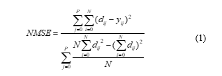 where P is the number of output processing elements (neurons), N is the number of exemplars in the data set, yij is the network output for exemplar i at processing element j, and dij is the desired output for exemplar i at processing element j. Since NMSE is an error term, values closer to zero denote better predictability. MSE is simply the numerator of NMSE.
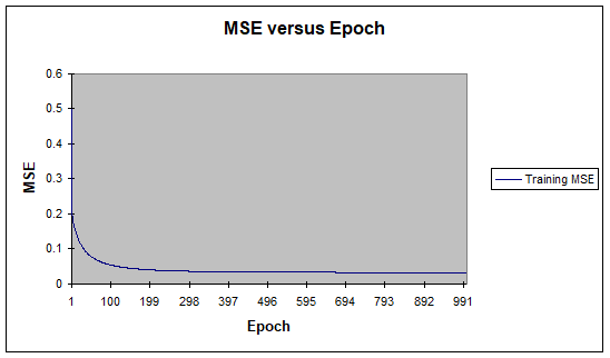
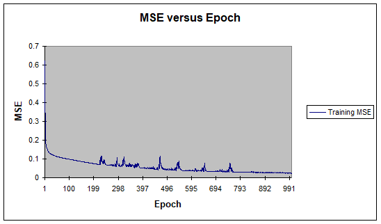 Figure 11: Mean Squared Error as (a) SVM and (b) ANN Training
Another statistically meaningful variable used for predictability performance is the correlation coefficient R. It is used to measure how well one variable fits on another, linear regression wise. In our case, these variables are predicted against the desired outputs. The R value is defined as:
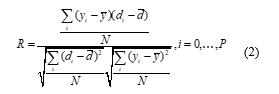 where y is the network output, and di is the desired output.
Table 4: Statistical Parameter Analysis and Comparison over Test Sets
The mean squared error (MSE) can be used to determine how well the network output fits the desired output, but it does not necessarily reflect whether the two sets of data move in the same direction. For instance, by simply scaling the network output, we can change the MSE without changing the directionality of the data. The correlation coefficient R solves this problem. By definition, the correlation coefficient between a network output y and a desired output d is defined by Eq. (4). The correlation coefficient is limited to the range [-1 1]. When R = 1, there is a perfect positive linear correlation between y and d; i.e., they vary accordingly. When R = -1, there is a perfect linear negative correlation between y and d;
i.e., they vary in opposite ways (when y increases, d decreases by the same amount). When R =0, there is no correlation between y and d; i.e., the variables are called uncorrelated. Intermediate values describe partial correlations.
We evaluate the performances of all classifiers in terms of sensitivity, specificity, accuracy, and precision. These parameters are statistical measures for classification. Values close or equal to 100% are desirable. They are related with true positive (TP), true negative (TN), false positive (FP) and false negative (FN) values, as explained below:
TP: Number of cases belonging to a certain class that are correctly classified.
TN: Number of cases not belonging to a certain class that are correctly classified.
FP: Number of cases belonging to a certain class that are incorrectly classified.
FN: Number of cases not belonging to a certain class that are incorrectly classified.
These parameters are calculated by the following equations:
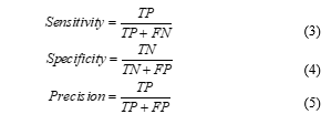
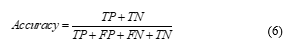 Table 5 shows the performance results of the classifiers adapting the proposed features on the basis of sensitivity, specificity, accuracy and precision. As can be seen, the performance of each classifier justifies that the visual features can be successfully employed in vowel classification. It is noted that the ANN and XGB classifiers perform better than the SVM. Since the XGB method is decision tree-based, and not a black-box, it is possible to see which features are more useful in the model as shown in Figure 12. In fact, this is a score that denotes the goodness of each feature during the building of the boosted decision tree model based on the splits. The more the feature is used in split decisions, the higher the score. The overall score for a feature is calculated as the average of the scores of that feature across all decision trees of the model.
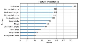 Figure 12: Feature Importance’s for XGB Model
In order to show the effectiveness of the offered visual features, the same vowel classes are also classified by utilizing the MFCCs, which are commonly used for speech recognition. Table 6 depicts the sensitivity results obtained from the proposed and MFCC features classified by all three classifiers. This table also includes the classification performance of the study in [7] which classifies the Turkish vowels by MFCCs using ANN.
It is fair to say that the proposed SV method yields better results, on average, on all classes with the exception of Class 2(E). It is observed that unlike the case of visual features, when MFCCs are used SVM performs slightly better than ANN and XGB.
Table 6: Comparison of Methods Using MFCCs and Proposed Visual Features
| Method |
Class 1(A) |
Class 2(E) |
Class 3(I-İ) |
Class 4(O-Ö) |
Class 5(U-Ü) |
| ANN (proposed visual features) |
100 |
73.68 |
100 |
84.62 |
93.55 |
| SVM (proposed visual features) |
100 |
54.17 |
100 |
80 |
86.21 |
| XGB (proposed visual features) |
100 |
93.33 |
100 |
80 |
87.88 |
| ANN (MFCC) |
83.33 |
80 |
66.67 |
57.14 |
63.63 |
| SVM (MFCC) |
85.71 |
80 |
77.78 |
66.67 |
60 |
| XGB (MFCC) |
50 |
70 |
60 |
60 |
90 |
| ANN Method in [7] (MFCC) |
88 |
81 |
76 |
78 |
81 |
Table 7: Comparison of Various Vowel Classification Studies
| Ref.No |
Language |
Input Features |
Clasifier |
Performance |
| 7 |
Turkish |
MFCC |
ANN |
80.8 |
| 29 |
Australian English |
Frequency Energy Levels |
Gaussian &ANN |
88.6 |
| 30 |
English |
MFCC |
SVM |
72.34 |
| 31 |
English |
Formant frequencies |
ANN |
70.5 |
| 32 |
English |
Formant frequencies |
ANN |
70.53 |
| 33 |
English |
Tongue and lip movements |
SVM |
85.42 |
|
34 |
Hindi |
MFCC |
HMM |
91.42 |
| 35 |
Hindi |
Gammatone Cepstral Coeficients + MFCC + Formants |
HMM |
91.16 |
| 36 |
Hindi |
Power Normalized Cepstral Coefficients |
HMM |
88.46 |
| Speech Vision (SV) |
Turkish |
Time Domain Visual Features |
ANN |
90,37 |
| SVM |
84,08 |
| XGB |
92,24 |
4.1. Comparison with Relevant Studies
In order to evaluate the performance of the SV approach more objectively, a literature search on various vowel classification performances is also carried out. In detail, a brief comparison is given in Table 6 with the results of another study; however, this study also contained Turkish vowels [7] whereas we are keen to look into the success rates of vowel classification in different other languages. On the other hand, it should be pointed out that the indirect comparison here is just to give a rough idea about the performance of the SV approach among other vowel classification results in general.
Harrington and Cassidy conducted a study on vowel classification in Australian English, using frequency energy levels with Gaussian and ANN classifiers [29]. Indeed, there are a number of studies classifying English vowels with SVM and ANN classifiers using MFCC and Formant Frequencies [30, 31, 32]. Another study was also conducted using tongue and lip movements to classify English vowels with SVM [33]. In addition, there are a few studies on vowel classification in the Hindi language using various frequency domain features and employing Hidden Markov Model (HMM) classifiers [34, 35, 36]. A comparison of these various studies with our SV approach, in terms of sensitivity, is given in Table 7.
5. Conclusion and Discussion
This paper describes a novel approach introducing visual features for classifying vowels. The proposed approach makes use of the geometric features obtained from speech waveform shapes. Shape-based features from speech signals have rarely been employed for speech recognition. On the other hand, the features that are widely used are usually in the transform domain, i.e. spectrograms. However, the techniques using spectrograms involve computational costs due to the Fourier transform calculations. In our approach, the recorded two-pitch long speech waveform is first processed to extract the visual features. For this purpose, the waveform is treated as an image. Therefore, several aforementioned image processing techniques are utilized. Then, the features are obtained from the processed waveform image. Finally, ANN, SVM, and XGB classifiers are trained for the vowels to be classified. The test results show that using visual features accomplish quite satisfactory performances.
It is fair to say, in comparison with the success rates of classical speech features; our speech vision approach introduces a promising performance. As it can be clearly seen in Table 7, it has the highest performance with the XGB classifier, which is slightly above 92%, among all the compared studies. Additionally, our neural network and SVM classifiers result in better or comparable scores with the others. Thus, it is clear that the proposed visual features work well for Turkish vowel classification.
These features can be used in applications where the visual part would make a difference such as in teaching hearing disabled individuals to speak. Although we applied the proposed features to Turkish vowels, it could be adapted to other languages easily, since the vowels in all languages share similar characteristics in the time domain. Combining both acoustic and visual features for vowel classification can be considered for future work.

 DOI: 10.25046/aj040303