1          Introduction

Recent household computers have high-performance processing schemes, e.g., multi-core, hyper-threading technologies and so on. Such parallel processing schemes enable the expansion of conventional applications to scientific and large amount of data processing applications in household computers. This transition increases the needs for parallel and distributed processing schemes, e.g., grid computing[1], utility computing and cloud computing[2]. These computing models require an appropriate execution method to acquire the optimal value in terms of the response time or the schedule length, energy consumption, the economic cost and throughput. However, to obtain the optimal schedule length has been an NP-complete problem. In a heterogeneous system where each processing speed and communication bandwidth is arbitrary, a task assignment method as well as a task scheduling method are needed because the actual processing time and communication time are determined after each task is assigned to a processor.

In various application models, especially for work-flow type application, called Directed Acyclic Graph (DAG) is one of currently studied task scheduling fields, also known as a DAG scheduling problem. DAG scheduling is classified into two approaches, i.e., list-based scheduling[3, 4, 5, 6] and clustering-based task scheduling[7, 8, 9, 10, 11]. In HEFT (Heterogeneous Earliest Finish Time)[3], which is the most famous list scheduling for DAG applications in heterogeneous systems, a scheduling priority is assigned to each task by using the average processing time and the average communication time. Then each task is assigned to a processor by which its completion time is minimized. Though the critical part of a list scheduling is how to define the priority for ready tasks, list-based scheduling models such as HEFT, PEFT[4] and CEFT[5] apply averaged processing time and communication time for deriving a priority value for each task. As a result, a good schedule length cannot be obtained if the job is data-intensive or has a large dispersion among task sizes and data sizes. On the other hand, in task clustering for heterogeneous systems, each task belongs to a task cluster. Each task cluster is assigned to a processor and each task is scheduled in order to minimize the schedule length. Though a task clustering method is known as one of the promising methods in homogeneous systems, a good schedule length cannot be obtained in heterogeneous systems because it assumes a temporal homogeneous system for deriving each clustering priority.

We proposed a task clustering method for heterogeneous systems for effective use of processors in [12], the

objective of which was to minimize the schedule length using a small number of processors. The method proposed in [12] firstly derives the lower bound of the total execution time of tasks in a cluster to regulate the number of processors. Then each task is clustered in order to minimize the schedule length by reducing the Worst Schedule Length (WSL). According to the literature in [13], minimizing WSL leads to the reduction of both the lower bound and the upper bound of the schedule length. Then each task is ordered by Ready Critical Path (RCP) scheduling[14] on each assigned processor. However, there is no criteria to minimize WSL in the task scheduling. In this paper, we propose a task scheduling to minimize WSL after the task clustering proposed in [12] has been finished. Experimental results in a real environment show that the proposed task scheduling outperforms the method in [12] in terms of the schedule length. This paper is an extension of work originally presented in the 19th International Conference on Advanced Communications Technology(ICACT2017)[15].

2          Assumed Model

2.1        Job Model

An assumed job is expressed as a Directed Acyclic Graph

(DAG), which is known as workflow type job. Let G = (V, E), where V is the set of tasks and E is the set of edges (data communications among tasks). An i-th task is denoted as n_i. Let w(n_i) be the workload of n_i, i.e., w(n_i) is the sum of unit times taken for being processed by the reference processor. We define the data dependency and direction of data transfer from n_i to n_j as e_i,j. And c(e_i,j) is the sum of unit times taken for transferring data from n_i to n_j over the reference communication link.

One constraint imposed by a DAG is that a task cannot be executed until all data from its predecessor tasks arrive. For instance, e_i,j means that n_j cannot be started until the data from n_i arrives at the processor that executes n_j. And let pred(n_i) be the set of immediate predecessors of n_i, and suc(n_i) be the set of immediate successors of n_i. If pred(n_i) = ∅, n_i is called START task, and if suc(n_i) = ∅, n_i is called END task. If there are one or more paths from n_i to n_j, we denote such a relation as n_i ≺ n_j.

2.2        System Model

We assume that each computer is completely connected to others, with non-identical processing speeds and nonidentical communication bandwidths. The set of processors is expressed as P = {p₁, p₂,…, p_n} and let the set of processing speeds in p_i be α_i. As for data communication among computers, let the communication bandwidth of p_i be β_i. Since the actual communication speed depends on the bottleneck in the network path, suppose the communication speed is the minimum value in the two bandwidths among p_i and p_j, i.e., L_i,j = min{β_i,β_j}, where L_i,j is the communication speed among p_i and p_j.

The processing time in the case that n_k is processed on p_i is defined as

t_p(n_k,α_i) = w(n_k)/α_i.                                   (1)

The data transfer time of e_k,l over β_i,j is defined as

t_c(e_k,_l, L_i,_j) = c(e_k,_l)/L_i,_j.                                 (2)

This means that both processing time and data transfer time are not changed with time, and suppose that data transfer time within one computer is negligible. In general, the communication setup time for the preparation, denoted by O_k occurs before p_k sends the data. If c(e_i,j) is sent from p_k to p_l, the communication time is defined by O_k and the communication speed L_k,l; in particular, L_k,l = min{β_k,β_l} and the communication time is given by t_c(e_i,_j, L_k,_l) = O_k + c(e_i,_j)/L_k,_l. (3)

We assume the communication setup time is negligible, i.e., O_k = 0 for ∀p_k ∈ P.

3          Related Work

In this section, we discuss existing methods for Directed Acyclic Graph (DAG) scheduling in heterogeneous systems. We also clarify their disadvantages when they are applied to systems with a large number of processors and when not all processors are used for execution. DAG scheduling for heterogeneous systems is categorized into two classes in terms of the task assignment policy: listbased heuristics [3, 4, 5, 16, 17] and task clustering [7, 8, 9, 10, 11].

For list-based heuristics, both HEFT[3] and Predict Earliest Finish Time (PEFT)[4] use the average processing time and average communication time to derive the scheduling priority for each free task whose predecessor tasks have been scheduled. According to the HEFT algorithm, the scheduling priority of task n_k is based on the path length from n_k to the END task, which is denoted by rank) as follows:

rank_u^∗(n_k) = t_p(n_k,α_i) + t_c(e_k,_l, L_i,_j)

+ max nrank_u^∗(n_l,α_j)^o.   (4) n_l∈suc(n_k)

In the set of free tasks, the task with the maximum rank_u value is chosen and assigned to the processor to minimize the completion time of the task using an insertion-based policy. PEFT[4] uses an Optimistic Cost Table (OCT); the OCT value of task n_k assigned to p_p is the longest path from n_k to the END task in the set of paths starting from n_k, provided that each path length assumes the minimum length in the processor assignment combinations when n_k is assigned to p_p. The scheduling priority of n_k in PEFT is the average OCT value of n_k through all of the processors in P. One difference between HEFT and PEFT is whether the actual processor assignment is considered during the prioritizing phase. Another difference is that PEFT uses the average value. In Constrained Earliest Finish Time (CEFT)[5], the pruning phase is performed first. In the pruning phase, the longest path, called the Constrained Critical Path (CCP), which is derived from the average processing time and average communication time, is pruned from the DAG. Then, the pruned DAG is traversed, and the new CCP is pruned. Pruning continues until all of the tasks are pruned. Tasks in a CCP are assigned to the same processor where their completion times are minimized. The Minimizing Schedule Length (MSL) algorithm[16] uses Mean Execution Time (MET) and Total Communication Time (TCT) for the scheduling priority derived by MET+TCT. They are calculated based on the average processing time and the average communication time. The Heterogeneous Selection Value (HSV) algorithm[17] derives rank_u^∗ values for all processors for each task. Then the average rank_u^∗ value is calculated as hrank_u. The scheduling priority in HSV is derived by the out degree times hrank_u, which reflects the idea that a task having larger out degree can have great effect on the schedule length. Since HEFT, PEFT, CEFT, MSL, and HSV use the average value calculated from all processor information, each scheduling priority is not accurate for minimizing the schedule length. Longest Dynamic Critical Path (LDCP)[6] uses the actual processing time and communication time for each scheduling priority and outperforms HEFT in terms of the schedule length. However, LDCP requires a set of DAGs for all processor assignment patterns, and thus, a high space complexity is required if the system has a large number of processors.

4          Overview of CMWSL Algorithm

In this section, we present an overview of the clusteringbased task scheduling, called CMWSL (Clustering for Minimizing Worst Schedule Length)[12]. CMWSL consists of: (i) the lower bound of the total processing time is derived to the processor by which the maximum worst schedule length (defined as WSL (Worst Schedule Length) in Section 4.1) is obtained. (ii) several tasks on WSL path are clustered until the total processing time exceeds the lower bound in order to minimize WSL. (iii) the execution order for each task on a processor is decided according to the scheduling priority. In the following sections, the definition of WSL, the lower bound, the task clustering procedures, and the task ordering procedures are presented. For more details, see the literature in [12].

4.1        WSL (Worst Schedule Length)

Since CMWSL assumes WSL, we present the basics of WSL. Intuitively, WSL is the maximum execution path length when each task is executed as late as possible in a node, provided that there is no data waiting time for each task once the node starts executing; that is, WSL is the upper bound of the schedule length if no data waiting time occurs for each processor.

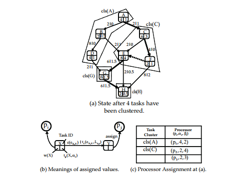
Fig. 1 shows an example of WSL derivation. In this figure, (a) is the state after four tasks have been clustered, (b) is the meaning for each items in (a), and (c) is the given system information, where three processors exist, i.e., p₁, p₂ and p₃. At (a), a virtual processor having the maximum processing speed (=4) and the maximum communication bandwidth (=4) is assumed to be assigned to a task. From this state, WSL is derived by A → C → F → E → G → H, i.e., the longest execution path length is obtained when E is scheduled as late as possible on p₂.

If a processor assignment can make WSL smaller, both the upper bound and the lower bound of the actual schedule length can be made smaller[13]. The schedule length cannot be obtained until every task execution order is determined. Thus, at the task clustering phase as a task assignment, the objective is to minimize WSL, not to minimize the actual schedule length.

4.2        Lower Bound of Total Execution Time for each Processor

In general, the more tasks are assigned to a processor, the more data communications can be localized on one processor. However, to increase the number of assigned tasks on a processor can lead to the reduction of the degree of parallelism. The balance between localization of data communication and parallelism should be considered for minimizing the schedule length. Furthermore, imposing the lower bound can reduce the number of assigned processors, thereby effective use of computational resources can be achieved. In CMWSL, the lower bound of the total processing time on a processor p_p is defined as follows (for more details, see the literature in [12]):

vuu_ut 1

δ_opt(α_p,β_p) =          ^              w(n_k) ,     (5) αp         αp                  

                    i

where

N

X                                 X     X

ε =                    w(n_k) −                         w(n_k),

n                       i

! cmax          cmax              wmin             cmin λ =   −              +              +              , βp               βmax             αmax             βmax

where seq^≺_s−1 be the set of tasks in a path from a START task to the END task in the WSL sequence at the workflow after

(s − 1) tasks have been clustered. In seq^≺_s−1, let seq^≺_s−1(i) be the set of tasks that belong to the i-th cluster. In addition, c_min and c_max are the minimum and maximum data sizes in seq^≺_s−1, and w_min is the minimum task size. Finally, α_max and β_max are the maximum processing speed and maximum communication bandwidth, respectively.

δ_opt(α_p,β_p) means the value when the upper bound of WSL is minimized. That is, both the lower bound and the upper bound of the schedule length is minimized by applying δ_opt(α_p,β_p) for each cluster.

Next, we present how the processor to which an assignment unit (we call it as “cluster”) is determined. CMWSL tries to find WSL path for each clustering procedure. On WSL path, there are two sub-paths, i.e., clustered path and unclustered path. Since tasks on a clustered path cannot be clustered anymore, the only set of tasks by which WSL can be varied is the unclustered path. Thus, on the unclustered path, the number of clusters whose total execution time exceeds δ (the variable for the lower bound), is defined as

                                                               

N  X≺− w(nk) −XN ∈ X≺− w(nk),               (6)

nk∈seqs 1                      i=1 nk seqs 1(i),

clss−1(i)<UEXs−1

(a)                  State after 4 tasks have been clustered.   Task Cluster Processor (pi ,α βi , i) cls A( ) (p 4 21, , ) cls C( ) (p 2 42, , ) (p3, , )2 3 (b)                  Meanings of assigned values.               (c) Processor Assignment at (a). Figure 1: Example of WSL Derivation

where δ = δ(α_p,β_p,G^s), G_s is the DAG after s tasks have been clustered, and α_pδ is the task cluster size of p_p. N(δ) is derived by taking the total workload of tasks on the unclustered path. Then, the increase of WSL by generating clusters by more r clustering steps on the unclustered path, is defined by

∆WS L^∗(M(G^s+r))

N(δ^∗)−y                                                             N(δ)

^X             up                                           ^X                up

≤                  ∆LVlnr(clss+r(i)) +                        ∆LVnlnr(clss+r(i))

i=1                                                          i=N(δ)−y+1

!

X         c(e_k,l)       c(e_k,l)

+                              −

e ∈seq≺ , Lp,q βmax k,l s−1 ^ek,l

≤ ∆WS L_up^∗ (M(G^s+r)),                                                        (7)

where ∆LV_lnr^up(cls_s+r(i)) is the increase of WSL by generating one linear cluster, i.e., all tasks in the cluster cls_s+r(i) has dependencies each other. ∆LV_nlnr^up (cls_s+r(i)) is the increase of WSL by generating one non-linear cluster, i.e., one or more tasks in the cluster cls_s+r(i) has no dependency with others. WS L )) is the upper bound of the increase of WSL, i.e., ∆WS L^∗(M(G^s+r)). δ_opt in (5), it is obtained by differentiating ∆WS L )) with respect to δ. Then ∆WS L )) takes the local minimum value when δ equals to δ_opt defined at (5).

From the set of unassigned processors, the processor having the minimum value of ∆WS L_up^∗ (M(G^s+r)) is selected as the next assigned target. In this phase, both the lower bound and the processor to be assigned to a cluster is determined.

4.3        Clustering Tasks

In the clustering phase, let the selected processor by the previous section be p_p. Then the actual lower bound, i.e., δ_opt(α_p,β_p) is derived. The unclustered task on WSL path becomes the start point for clustering. From such a task, the successor tasks are included in the same cluster until the total processing time exceeds δ_opt(α_p,β_p) in order to minimize WSL.

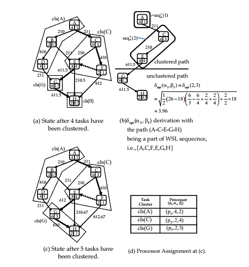
Fig. 2 shows an example of the task clustering phase in CMWSL. In this figure, (a) is the state after four tasks have been clustered, which is the same state as (a) at fig. 1. (b) in fig. 2 is the path on WSL path, i.e., A, C, E, G, H. In this path, the clustered path is A → C → E, and the unclustered path is G → H. Thus, G becomes the start point for the next

task clustering and p₃ is selected as the next assignment target, because only p₃ remained as the unassigned processor. From this state, the lower bound, i.e., δ_opt(α₃,β₃) ≈ 3.96. Then at (c), G and H are clustered as a cluster cls(G). Since the total processing time is 3+1 > 3.96, no more task are included at cls(G). The clustering phase is finished if all clusters are generated with exceeding each lower bound.

5          Task Ordering

Task Cluster Processor (pi ,α βi , i) cls A( ) (p 4 21, , ) cls C( ) (p 2 42, , ) cls G( ) (p3, , )2 3 been clustered.              the path (A-C-E-G-H)      being a part of WSL sequecnce,             i.e., A,C,F,E,G,H {      } (c) State after 5 tasks have (d) Processor Assignment at (c). been clustered. Figure 2: Example of Task Clustering in CMWSL

In this section, we present two list-based task ordering criteria in CMWSL. One of the objectives of this paper is to determine which one is better for minimizing the schedule length. Thus, the task ordering phase is performed after the task clustering phase presented in Section 4.3. In this phase, determining the actual execution order for each task is performed. Since the assigned processor for each task is known, the objective in this phase is to minimize the schedule length, not WSL. According to the literature in [18], a list-based task ordering method was proposed, where the task in the current WSL sequence is selected from the free list. Here, “free list” is the set of tasks, whose all immediate predecessor tasks have already been scheduled. We shall call the task ordering method as “List maxLV”. The fundamental idea behind List maxLV is that the task in WSL sequence can have an effect on the worst schedule length, i.e., such a task can prolong the actual schedule length depending on the execution ordering. Thus, such a task must be scheduled as early as possible. The task ordering method in CMWSL is quite different. The task ordering in CMWSL selects the task having the minimum DRT (data ready time) from the free list. DRT of task n_j on p_q is defined as

DRT(n_j, p_q) = max                nt_f (n_i, p_p) + t_c(c(e_i,_j), L_p,_q)^o,      (8)

n_i∈pred(n_j), p_p∈P

where t_f (n_i, p_p) is the finish time of n_i on p_p, and n_j on p_q is supposed to reveive the data from n_i on p_p. We shall call the ordering method as “List minDRT”.

Fig. 3 demonstrates behaviors of both List minDRT and List maxLV. In this figure, A, B, and C are supposed to have been already scheduled. Thus, the content of the free list is {E, F,G}. In List minDRT, DRTs of E, F, G are supposed to be 14, 16, and 6, respectively. Then G, having the minimum DRT is selected for assigning an idle time slot. In List maxLV, the priority is defined as “level”, which is the longest execution path length when the task is scheduled as late as possible. In this case, level values of E, F, and G are supposed to be 24, 12, and 23, respectively. Thus, E is selected because its level value is the maximum.

6          Experiment

In this section, we present the comparison results in terms of the response time as the speed-up ratio in a realistic environment. The objective of this paper is to confirm the performance of CMWSL in the real environment for practical use of CMWSL, as well as which list-based task ordering policy is better in List minDRT and List maxLV. We adopt Gaussian Elimination DAG and FFT (First Fourier Transform) DAG as target DAGs.

6.1        Comparison Target

As for task ordering methods in CMWSL, we adopt List minDRT and List maxLV. We name List minDRT in CMWSL as “CMWSL DRT”, and List maxLV in CMWSL as “CMWSL LV”. As other comparison targets, HEFT[3], CEFT[5], HSV[17], and PEFT[4] are adopted, because these heuristic algorithms are known to derive a good schedule length with low time complexity, i.e., they are applicable in a real situation.

6.2        Gaussian Elimination DAG

In this comparison, we prepared 20 nodes that were connected in the local network as a heterogeneous cluster. Ta-

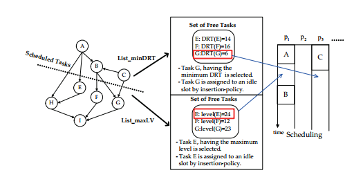Figure 3: Example of Task Ordering Methods Table 1: Specification of the Experimental Environment for Gaussian Elimination DAGs. Node ]         CPU Freq.          tproc (µs)            αp                       Bandwidth        tcomm (µs)            βp 1 300MHz 0.157 1.00 100Mbps 2.27 1.00 2 533MHz 0.136 1.16 1Gbps 0.45 5.04 3 800MHz 0.091 1.74 100Mbps 2.15 1.06 4 1.0GHz 0.057 2.74 1Gbps 0.62 3.66 5 1.2GHz 0.051 3.06 1Gbps 0.33 6.88 6 1.5Ghz 0.038 4.14 100Mbps 2.03 1.12 7 1.5Ghz 0.035 4.45 1Gbps 0.55 4.13 8 2.0GHz 0.032 4.92 1Gbps 0.34 6.68 9 2.4GHz 0.029 5.49 100Mbps 0.38 5.97 10 2.4GHz 0.027 5.76 1Gbps 0.27 8.41 11 2.6GHz 0.025 6.21 1Gbps 0.42 5.40 12 2.6GHz 0.024 6.56 100Mbps 2.2 1.03 13 2.8GHz 0.022 7.15 1Gbps 0.22 10.32 14 2.8GHz 0.021 7.61 1Gbps 0.37 6.14 15 2.8GHz 0.021 7.61 100Mbps 1.89 1.20 16 2.8GHz 0.019 8.43 1Gbps 0.28 8.11 17 3.0GHz 0.016 9.83 1Gbps 0.29 7.83 18 3.0GHz 0.015 10.26 1Gbps 0.39 5.82 19 3.0GHz 0.015 10.26 100Mbps 2.11 1.08 20 3.2GHz 0.013 12.42 1Gbps 0.21 10.81

ble 1 presents the specifications of the environment in terms of processing and communication performance for Gaussian elimination DAGs. In this table, t_proc represents the time taken to process one arithmetic operation, and t_comm is the time taken to send one byte from the node to the router in the local network. In particular, t_comm was derived by RTT/(] of bytes ∗ 2) of pinging.

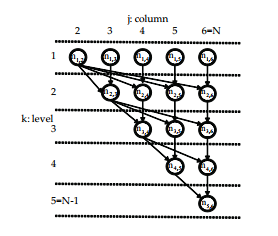
As for the DAG structure, we consider one task as a second inner loop, i.e., for(j = k + 1; j ≤ N; j ++) at the kji Gaussian elimination without pivoting. That is, the same as the one in Section 5.5.1. Fig. 4 presents one example of Gaussian elimination DAG at N = 6. According to the study in [19], the processing time of a task n_k,j and the communication time of a data point c(e_{(k,j),(k+1,m)}) are defined as follows:

w(n_k,_j) = (2(N − k) + 1)t_proc,

c(e(k,j),(k+1,m)) = Op + (N − k + 1)tcom,                 (9)

where O_p is the setup time of p_p performed before sending data, t_proc is the processing time for one arithmetic operation, and t_com is the communication time per

byte. This model was proved to be asymptotic to a real environment[19]. Then, we can rewrite (9) using t_c(n_k,j,α_p)

and t_c(c(e_(k,_j),_(k+1,_m)), L_p,_q)), as follows:

(2(N − k) + 1)t_proc t_p(n_k,_j,α_p) =    ,

tc(c(e(k,j),(k+1,m)), Lp,q) = Op + (N − k + 1)               ,

Lp,q

(10)

where t_proc and t_comm are the values obtained by the reference processor. α_p is the processing speed ratio when that of the reference processor is equal to one, and L_p,q is the communication bandwidth ratio when the reference communication bandwidth is equal to one.

Figure 4: Gaussian Elimination DAG at N = 6. Figure 5: Comparison of Speed-Up Ratio for Gaussian Elimination DAGs in a Real Environment.

First, we executed the simulation using the information listed in Table 1.^[1] We obtain the mapping of a task and a processor through the results of the simulation. Then, we implemented the parallelized MPI (MPICH2[20]) program with non-blocking communication in the C language by hand-coding each algorithm. For each algorithm, the program was executed 100 times, and we averaged the speedup ratio defined by the schedule length of “node 20” in Table 1, divided by that of each algorithm.

Fig.             5 presents the results in cases of N = 50 and

N = 100. CMWSL-DRT and CMWSL-LV outperform the other algorithms in both cases (N = 50 and N = 100). We can see that PEFT, CEFT, and HSV output a smaller schedule length than HEFT. In the real environment, the setup time is nonzero for each processor, and therefore the communication time can have a greater effect on the schedule length than in the simulation. Even in such a case, both CMWSL-DRT and CMWSL-LV have a smaller schedule length than the other algorithms. As for the comparison between CMWSL-DRT and CMWSL-LV, it is observed that CMWSL-DRT outputs better speed-up ratio. In CMWSLLV, a task, e.g., n_k by which WSL is obtained if it is scheduled as late as possible, is selected from the free list. However, even if n_k is selected, the actual schedule length cannot be made smaller if n_k is not a critical task, i.e., n_k does not belong to the actually dominating execution path in terms of the schedule length. In CMWSL-DRT, selecting a task having the minimum DRT can lead to the actual schedule length; that is, scheduling a task, e.g., n_k having the minimum possible start time can reduce the data waiting time from n_k. As a result, the total idle time for each processor can be suppressed.

6.3        FFT DAG

In FFT DAG, every task size is equal and every data size is equal. The FFT DAG used in this comparison contains mlogm butterfly operation tasks, where m is the matrix size, as in Section 5.5.2. Each task contains the following operations:

y(k)	=	ye(k) + ωk ∗ yo(k),0 ≤ k ≤ m/2 − 1,
y(k + m/2)	=	ye(k) − ωk ∗ yo(k),0 ≤ k ≤ m/2 − 1,

(11)

where y_e is the FFT of even points and y_o is the FFT of odd points. That is, every task involves the same number of operations. Although the data size among all tasks is the same, it contains both the real and imaginary parts as double type variables. Thus, we define each data size as 16 bytes.

Table 2 presents the specification of the environment in terms of processing and the communication performance for FFT DAGs. In this table, the “Task Size” is measured by executing (11) for each processor, while the “Data Size” is defined by multiplying t_comm from Table 1 by 16. From this information, α_p and β_p are derived for the simulation. Similar to the case of Gaussian elimination DAGs, we obtain the mapping of each task and each processor from the results of the algorithms in the simulation. Then, we implemented the parallelized MPI program with non-blocking communication in the C language.

Fig. 6 presents the comparison results in cases of m = 128 and m = 256, in terms of the speed-up ratio. In both cases, both CMWSL-DRT and CMWSL-LV outperform the other algorithms. However, the differences of the speed-up ratio between CMWSL (CMWSL-DRT and CMWSL-LV) and the other algorithms are not large compared with the case of Gaussian elimination, as seen in Fig. 5. As for the comparison between CMWSL-DRT and

Table 2: Specification of the Experimental Environment for FFT DAGs. Node ]         CPU Freq.          Task Size (µs)            αp                       Bandwidth         Data Size(µs)           βp 1 300MHz 37.540 1.00 100Mbps 36.32 1.00 2 533MHz 17.114 2.19 1Gbps 7.2 5.04 3 800MHz 13.736 2.73 100Mbps 34.4 1.06 4 1.0GHz 8.438 4.45 1Gbps 9.92 3.66 5 1.2GHz 7.757 4.84 1Gbps 5.28 6.88 6 1.5Ghz 6.672 5.63 100Mbps 32.48 1.12 7 1.5Ghz 6.231 6.02 1Gbps 8.8 4.13 8 2.0GHz 4.003 9.38 1Gbps 5.44 6.68 9 2.4GHz 3.822 9.82 100Mbps 6.08 5.97 10 2.4GHz 3.539 10.61 1Gbps 4.32 8.41 11 2.6GHz 3.221 11.65 1Gbps 6.72 5.40 12 2.6GHz 3.183 11.79 100Mbps 35.2 1.03 13 2.8GHz 3.105 12.09 1Gbps 3.52 10.32 14 2.8GHz 2.994 12.54 1Gbps 5.92 6.14 15 2.8GHz 2.944 12.75 100Mbps 30.24 1.20 16 2.8GHz 2.919 12.86 1Gbps 4.48 8.11 17 3.0GHz 2.896 12.96 1Gbps 4.64 7.83 18 3.0GHz 2.863 13.11 1Gbps 6.24 5.82 19 3.0GHz 2.732 13.74 100Mbps 33.76 1.08 20 3.2GHz 2.556 14.69 1Gbps 3.36 10.81 Figure 6: Comparison of Speed-Up Ratio for FFT DAGs in a Real Environment.

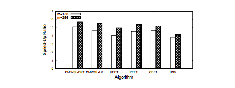
CMWSL-LV, CMWSL-DRT outputs better results in both cases (m = 128,256). Similar to the result obtained in Section 6.2, selecting a task having the minimum possible start time can contribute to reduce the data waiting time for each processor. In general, the data size among tasks in FFT DAG is smaller than that in Gaussian Elimination DAG. This means that the effect of the communication delay is smaller in case of FFT DAG. Thus, the difference of schedule length among algorithms is also small.

From these results, we can infer that CMWSL can be applied to the FFT in a real environment.

7          Conclusion and Future Works

In this paper, we confirmed the performance and behaviors of CMWSL in a real environment using Gaussian Elimination and FFT program. According to the obtained results, CMWSL outperforms other list-based task scheduling algorithms in terms of the speed-up ratio, i.e., the schedule length. We also presented the comparison results among two task ordering methods, i.e., List minDRT and List maxLV for CMWSL. In CMWSL, List minDRT was proved to output a better result than List maxLV. That is, we can say that the task having the minimum possible start time should be selected for scheduling.

[1] O_p depends on many factors, including the program coding style and the processor status at the execution. This makes it difficult to specify O_p for each processor. We fixed the setup time O_p=0 in the simulation.

1. I. Foster, “The Grid: A new infrastructure for 21st century science,” Physics Today, Vol.55(2), pp. 42–47, 2002.
2. S. Di and C.L. Wang, “Dynamic Optimization of Multiattribute Resource Allocation in Self-Organizing Clouds,” IEEE Trans. Parallel Distrib. Syst., Vol. 24, No. 3, pp. 464-478, 2013.
3. H. Topcuoglu, S. Hariri, M. Y. Wu, “Performance-Effective and Low-Complexity Task Scheduling for Heterogeneous Computing,” IEEE Trans. Parallel Distrib. Syst., Vol. 13, No. 3 pp. 260-274, 2002.
4. H. Arabnejad and J. G. Barbosa, “List Scheduling Algorithm for Heterogeneous Systems by an Optimistic Cost Table,”, IEEE Trans. Parallel Distrib. Syst., Vol. 25, No. 3, pp. 682-694, 2014.
5. M. A. Khan, “Scheduling for heterogeneous systems using constrained critical paths, ” Parallel Comput., Vol. 38, No. 4-5, pp. 175-193, 2012.
6. M. I. Daoud and N. Kharma, “A high performance algorithm for static task scheduling in heterogeneous distributed computing systems,” J. Parallel Distrib. Comput., Vol. 68, No. 4, pp. 399–409, 2008.
7. A. Gerasoulis and T. Yang, “A Comparison of Clustering Heuristics for Scheduling Directed Acyclic Graphs on Multiprocessors,” J. Parallel Distrib. Comput., Vol. 16, pp. 276-291, 1992.
8. B. Jedari and M. Dehghan, “Efficient DAG Scheduling with Resource-Aware Clustering for Heterogeneous Systems,” Comp. Inf. Sci., Vol. 208, pp. 249–261, 2009.
9. S. Chingchit et al., “A Flexible Clustering and Scheduling Scheme for Efficient Parallel Computation,” in Proc. of the 13th Int. Parallel Distrib. Process. Symp., pp. 500–505, 1999.
10. C. Boeres et al., “A Cluster-based Strategy for Scheduling Task on Heterogeneous Processors,” Proc. of the 16th Symp. on Comp. Arch. High Perform. Comput. (SBAC-PAD’04), pp. 214–221, 2004.
11. B. Cirou and E. Jeannot, “Triplet: a Clustering Scheduling Algorithm for Heterogeneous Systems,” in Proc. Int. Conf. on Parallel Process. Workshops (ICPPW’01), pp. 231–236, 2001.
12. H. Kanemitsu , M. Hanada, and H. Nakazato, “Clustering-based task scheduling in a large number of heterogeneous processors,” IEEE Trans. Parallel Distrib. Syst., Vol. 27, No. 11, pp. 3144–3157, 2016.
13. Hidehiro Kanemitsu, Gilhyon Lee, Hidenori Nakazato, Takashige Hoshiai, and Yoshiyori Urano, “On the Effect of Applying the Task Clustering for Identical Processor Utilization to Heterogeneous Systems,” Grid Comput., pp. 29 – 46, 2012.
14. T. Yang and A. Gerasoulis., “List scheduling with and without communication delays,” Parallel Comput., pp. 1321 – 1344, 1993.
15. S. Hashimoto, E. H. Weyulu, K. Hajikano, H. Kanemitsu, and M. W. Kim, ”Evaluation of Task Clustering Algorithm by FFT for Heterogeneous Distributed System”, in Proc. the 19th Int. Conf. Adv. Comm. Tech.(ICACT2017), pp. 94-97, 2017.
16. D. Sirisha and G. V. Kumari, “A new heuristic for minimizing schedule length in heterogeneous computing systems,” in Proc. IEEE Int. Conf. on Elect. Comput. and Comm. Tech. (ICECCT), pp. 1–7, 2015.
17. G. Xie et al., “Heterogeneity-driven end-to-end synchronized scheduling for precedence constrained tasks and messages on networked embedded systems, ” J. Parallel Distrib. Comput., Vo. 83, pp. 1–12, 2015.
18. H. Kanemitsu and M. Hanada, ”A Task Scheduling with Response Time Estimation for Efficient Processing in Heterogeneous Systems,” in Proc. of 2015 RISP Int. Work. Nonlinear Circuits, Comm. Sig. Process. (NCSP 2015), 2015.
19. A. K. Amoura et al., “Scheduling Algorithms for Parallel Gaussian Elimination with Communication Costs,” IEEE Trans. Parallel Distrib. Syst., Vol. 9, No. 7, pp. 679–686, July 1998.
20. MPICH web site: https://www.mpich.org/ .

(Click to view)

(Click to view)