Energy-Efficient Mobile Sensing in Distributed Multi-Agent Sensor Networks

Adv. Sci. Technol. Eng. Syst. J. 2(3), 245–253 (2017);
 DOI: 10.25046/aj020334
In this paper, we exploit an integration between Compressive sensing (CS) and the random mobility of sensors in distributed mobile sensor networks (MSNs). A small number of distributed mobile sensors are deployed randomly in a sensing area to observe a large number of positions. The distributed mobile sensors sparsely sample the sensing area for data collection. At each sampling time, the sensors collect data at their random positions and exchange their readings to the others through their neighbors within the sensor transmission range to form one CS measurement at each sensor. After a certain number of rounds for moving, sensing and sharing data, each mobile sensor creates a sufficient CS measurements to be able to reconstruct all readings from all positions that need to be observed. Network performance is analyzed considering the number of sensors deployed in the networks, the convergence time and the sensor transmission range. Expressions for transmission power consumption are formulated and optimal low power cases are identified.
1. Introduction
Energy efficiency is the most important issue for mobile sensor networks (MSN) that can be useful for measuring data in many applications including environmental monitoring, event detection, intrusion detection, etc. These networks are constructed from sensors, control algorithms and other dynamic factors which depend on specific purposes or application scenarios [1, 2]. We define the vector X = [x1x2…xN ]T to represent all sensor readings from the locations to be observed. These readings are typically highly correlated and compressible and could be an object for energy saving.
Compressive sensing (CS) [3, 4, 5] offers to sample and to reconstruct sparse or compressible signals using fewer samples than the Nyquist-Shannon theorem would suggest. CS can be applied effectively with wireless sensor networks (WSN) and MSNs to reduce the amount of data and power required by the network. The technique can recover all data from X based on a small number of CS measurements (Y = [y1y2…yM]T ) compared to the number of nodes or positions (M N) as Xˆ = arg min k X k1 , subjectto Y = ΦX, where Φ is the measurement matrix, also called routing matrix in wireless networks. Each CS measurement can be collected from all sensing nodes or from some random nodes.
In this paper we propose a novel frame work that exploits CS sampling by mobile sensors deployed randomly in a sensing area. At each sampling time, each sensor samples its own data as xi which is shared with others L connected sensor nodes in the MSN. We assume the mobile sensors move into random positions in the area. After each round of moving, data sampling, and sharing, a linear combination of readings is computed as yi = PLj=1xj. To achieve a desired errortarget, each mobile sensor needs to move M times and share data to obtain M CS measurements (Y ∈ RM). A CS recovery algorithm can be applied to reconstruct all readings from positions in the sensing area (Xˆ ∈ RN ).
With a set transmission range, R, mobile sensors may move out of range and become disconnected from the group. With the proposed method the unequal CS measurements do not negatively impact CS performance due to a sparse binary measurement matrix.
1.1 Related work
The integration between CS and data collection methods in WSNs is being exploited effectively [6, 7]. It offers to reconstruct all readings from the networks based on a small number of CS measurements. Each CS measurement is collected from some random sensors. Some data collection methods utilizing CS are proposed as energy efficient algorithms to reduce power consumption for sensors. In [8, 9, 10] random walks with CS provide distributed routing methods for WSNs. Cluster based [11, 12] and tree based [13, 14] data collection methods significantly show the power reduced based on the combination with CS.
Recent research studies have exploited the mobility of sensors and CS. Wang [15] applied CS to monitoring vehicle networks. Mostofi built maps in mobile networks [16] and robot networks [17] while the mobile sensors and robots were deployed outside the sensing areas. Huang [18] reconstructed a scalar field using MSNs and information fusion. Nguyen [19, 20] used flocking control to lead a group of distributed robots to sample data and applied CS to recover data from the field based on a certain number of CS measurements.
The previous work has not focused on the integration between the random mobility of sensors and CS. In this paper, we complete our previous work [21]. The mobile sensors move only a certain number of times and share data among them to generate a desired number of CS measurements. Each sensor can reconstruct all raw data based on the measurements. The important results in this paper include:
- A proposed new distributed compressive mobilesensing data collection method.
- Formulations and analysis for estimating networktransmission power consumption.
- Analysis and simulation of factors such as the number of mobile sensors, the convergence time and the sensor transmission range leading to choices of minimizing power consumption.
2 Problem Formulation
2.1 Network Model
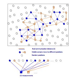
We assume an area to be observed with N unknown positions corresponding to N readings for collection. There are L mobile sensors randomly distributed in the sensing area to sense data. They are allowed to move with random direction and random velocities. The connections between sensors are created by radio links having a maximum sensor transmission range denoted as R. An appropriate value of R is chosen for all sensors. As shown in Figure 1, all mobile sensors are connected as an undirected graph G(L,E), where L is the set of vertices representing the mobile sensors and E is the set of edges representing the connections between sensors.
We further assume that the distributed sensors move randomly in the area. Each mobile sensor shares data to the others through its neighbors within the transmission range R.
2.2 Compressive Sensing (CS)
Compressed Sensing techniques [3, 4, 5] bring us amazing work to recover a compressible signal from undersampled random projections. They are also called measurements. A compressible vector signal X ∈ RN (X = [x1x2…xN ]T ) is k-sparse (X has k non zero elements) or dense but sparse in Ψ domain X = ΨΘ (where Θ is k-sparse vector) will be sampled and then recovered precisely with CS algorithm. The huge gain when we apply CS is the number of measurements are much less than the number of original vector values. Vector Y, called the measurement vector, contains data sampled from N sensor readings;
Y ∈ RM (Y = [y1y2…yM]T ), where M N.
Signal Sampling: The random measurements are generated by Y = ΦX where Φ ∈ RM×N is often fullGaussian matrices or binary matrices, called projection matrices. Y ∈ RM is the measurement vector with yi = Pnj=1ϕi,jxj, where ϕi,j are all entries on the ith row of our projection matrix Φ.
Signal Recovery: The number of CS measurements required to reconstruct the original signal perfectly with high probability is M = O (klog N/k) following the l1 optimization problem given by [3].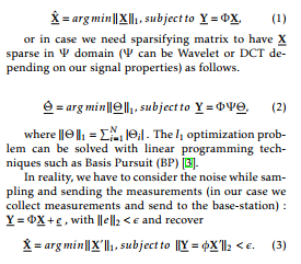
2.3 Data Collection in Distributed MSNs utilizing CS
The idea of applying CS into MSNs is that the sensing field can be sampled randomly based on the mobility of mobile sensors randomly deployed in the field. In general, each CS measurement is a collection from some random positions as shown in Figure 2. L mobile sensors are deployed randomly in the sensing area that they can collect sensing data randomly. If these sensors exchange their own data to each other, they can all achieve the data sampled randomly as shown in Figure 2
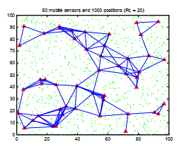
randomly as shown in Figure 2. At this point, one CS measurement is collected at each distributed mobile sensor. After M moving steps, each sensor has M measurements. This number of measurements defined in CS background in Section 2.2 helps to reconstruct all sensory readings from N positions in the area.
After M periods of time, L distributed mobile sensors visit approximately N unknown positions. The readings are contained in vector X which is compressible or sparse in proper domains as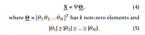
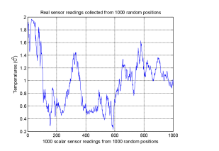
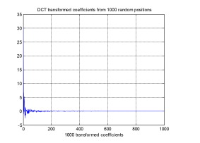
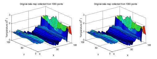
Ψ referred to as the sparsifying matrix, is an orthogonal basis of RN . If X is a k-sparse vector, Ψ is an identity matrix. Otherwise, Ψ can be chosen from another domain such as wavelet, DCT (discrete cosine transforms), etc. In order to verify this problem, Figures 3 and 4 are provided. All raw sensor readings from 1000 points of interest are shown in Figure 3. This real data is not sparse but it is highly correlated due to the positions next to each other. DCT Ψ matrix has been chosen to sparsify the real data. Figure 4 shows all the coefficients in DCT domain. We can see that signal energy would be reduced following Equation 5.
At time instant t, mobile sensor l at position i collects sensory data xil (i = 1, … N). All L mobile sensors share their readings (xil), identified by the corresponding position indices, with the other mobile sensors through their neighbors as shown in the graph G(L,E). After a convergence time, denoted as I, each mobile sensor has one CS measurement as a sum of L sensor readings![]()
where et is additive noise dependent on the system. φti is a binary vector (dimensioned 1 × N) that represents which positions are sampled at time instant t. It is also the tth row in the measurement matrix ΦM×N after M periods of time. The total measurements collected at each sensor are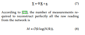
where k < M N. So instead of collecting N readings, one for each sampling position in the sensing area, each mobile sensors needs only M measurements and reconstructs all data from the area. If the network is fully connected all the time, each sensor has the same binary measurement matrix Φ with a constant row weight of L.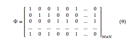
The restricted isometry property (RIP) of the sparse binary matrix has been studied in [23] where it is shown that the matrix can satisfy RIP and therefore can be used as an efficient measurement matrix. This matrix (ΦM×N ) can perform as well as a full Gaussian matrix for the CS recovery process. is set as <k e k2. The recovery algorithm is addressed as![]()
3 CompressiveMobileSensingAlgorithm (CMS)
for t = 1 to M do
- distributed mobile sensors move and sample a sensing area at M periods of time,
and create 1 CS measurement at each time instant t
while (Number of times sharing data < I) do for i = 1 to L do
Each sensor out of L mobile sensors has two main activities:
- send/receive data to/from neighbors
- add/forward new received data from/to neighbors
end
New data is detected by its attached
indices
One CS measurement is created following
end
- CS measurements are created for the CS data reconstruction following Eq. 10
Algorithm 1: CMS Algorithm
As mentioned, each distributed mobile sensor must collect M measurements to be able to reconstruct all readings from N positions in the sensing
area. With L distributed mobile sensors fully connected as given by the graph G(L,E) and based on the sensor transmission range R, the proposed algorithm is summarized as Algorithm 1.
Due to the limitation of R and sensor motion, some mobile sensors maybe disconnected from others and separated at time instant t + k. This means that the measurements yt+k collected at each sensor are not from all L sensors. This does not affect CS performance when the measurement matrix has different row weights [22]. By applying CS, each mobile sensor only has to visit M positions to collect all data from the sensing area (M N). This significantly reduces consumed power not only for communications but also for sensor movements.
4 Analysis of Power Consumption for Communications
The total consumed power for communications in the network consists of three main elements: the intraneighborhood consumed power denoted as Pnei, the convergence time I and the number of measurements required (M). The total power consumption can be calculated as follows![]()
Pnei represents the communication cost associated with L mobile sensors transmitting data to their neighbors and can be calculated as![]()
where ω is the average number of neighbors of each sensor corresponding to the available communication links, and α is the path loss exponent. It is shown in [24] that α = 2 and α = 4 for free space and multipath fading channels, respectively. We choose α = 2 throughout this paper. In the following sections both circular and square sensing areas are examined and analyzed.
4.1 Circular Sensing Area
If sensors are randomly distributed in a circular sensing area with radius R0, the average number of sensors deployed in the area covered by each sensor transmission range R can be found as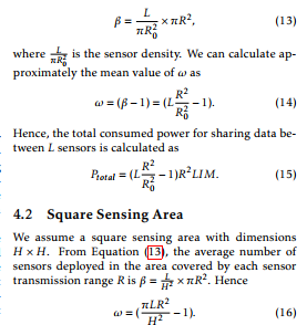
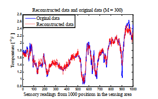
In Figure 6, both the true and the reconstructed data are shown together to illustrate the accuracy of the CS recovery algorithm with the number of CS measurements given by M = 300 stored at each sensor. The larger the number of measurements, the better the accuracy of the reconstruction.
The total consumed power for sharing data for L sensors to achieve M converged CS measurements in the square sensing area can be written as![]()
convergence time I depends on both the sensor density (πRL20 or HL2) and the connections between the sensors. The smaller the number of mobile sensors, the smaller the convergence time. However, since the transmission range R determines the connections, increasing the transmission range R to maintain the connections increases the transmission power consumption. This means that increasing or reducing R may
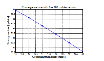
ing area and transmission range R∗ = 15.
increase or reduce the number of connections between the sensors in each neighborhood. Increasing the connections between sensors reduces the convergence time I. Thus a trade-off exists between these various parameters.
5 Simulation Results
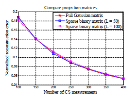
Figure 5 compares the ability to reconstruct data in the CS recovery process between three measurement matrices. Both sparse binary matrices with row weight L = 50 and 100 are shown to perform as well as the full Gaussian matrix which corresponds to full sampling.
We assume a fixed number of 50 or 100 mobile sensors deployed in a square sensing area of 100 square units (H = 100). We also assume that there are approximately 1000 positions where temperature needs to be observed. We consider the transmission range of 15 ≤ R ≤ 20 units in which the network is always connected. Without loss of generality, it is assumed that the power for transmitting 1 unit of data is 1 unit of power. The simulations were performed using real temperature sensor data from Sensorscope [25]. The reconstruction error related to CS signal recovery is the normalized reconstruction error given as kXkX−Xkˆ2k2.
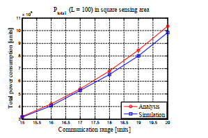
Figure 7 illustrates that as R is increased, the convergence time I is reduced as discussed in Section 4. Figure 8 depicts the corresponding total power consumption in the network, and we see the power consumption is reduced as R is decreased. R cannot be reduced without limit as at some point the L sensors will become disconnected and fragmented resulting in an excessively sparse measurement matrix.
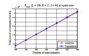
We chose the smallest transmission range R∗ = 15 and the corresponding convergence time I∗ = 94 for the optimal total power consumption for sensor communications in the network in both analysis and simulation which are shown in Figure 9.
Finally, in Figure 6, both the true and the reconstructed data are shown together to the show the accuracy of the CS recovery algorithm at the number of CS measurements as M = 300 stored at each sensor. The more number of measurements, the better accuracy of the reconstruction.
6 Conclusions and Future Work
This paper proposed a framework for distributed MSNs utilizing CS for efficient data sensing and recovery and investigated the dependence of power consumption on various MSN parameters. The algorithm exploits the random mobility of sensors for sparse sampling the sensing area. CS based sampling and reconstruction of the sensory data with a sparse binary measurement matrix were compared with dense Gaussian and shown to be equal under the simulation conditions, illustrating that CS may be used to advantage in MSNs. Expressions for transmission power consumption in the MSN were developed, simulated, and analyzed. The results show the trade-off between the number of sensors, the transmission range, and the convergence time that can further reduce the power consumption for data transmission in the networks.
In future work, we consider the correlation of sensing data in the field. This could help to improve the performance of CS in signal recovery.
Acknowledgment This work is supported by Thai Nguyen University of Technology (TNUT), Viet Nam.
- B. Liu, O. Dousse, P. Nain, and D. Towsley, “Dynamic coverage of mobile sensor networks,” Parallel and Distributed Systems, IEEE Transactions on, vol. 24, pp. 301–311, Feb 2013.
- C. Tunca, S. Isik, M. Donmez, and C. Ersoy, “Distributed mobile sink routing for wireless sensor networks: A survey,” Communications Surveys Tutorials, IEEE, vol. 16, pp. 877–897, Second 2014.
- D.L.Donoho, “Compressed sensing,” Information Theory, IEEE Transactions on, vol. 52, pp. 1289 –1306, 2006.
- E. Candes, J. Romberg, and T. Tao, “Robust uncertainty principles: exact signal reconstruction from highly incomplete frequency information,” Information Theory, IEEE Transactions on, vol. 52, pp. 489 – 509, Feb. 2006.
- E. Candes and J. Romberg, “Sparsity and incoherence in compressive sampling,” Inverse problems, vol. 23, no. 3, p. 969, 2007.
- G. Quer, R. Masiero, G. Pillonetto, M. Rossi, and M. Zorzi, “Sensing, compression, and recovery for wsns: Sparse signal modeling and monitoring framework,” Wireless Communications, IEEE Transactions on, vol. 11, pp. 3447–3461, October 2012.
- M. T. Nguyen, K. A. Teague, and N. Rahnavard, “Ccs: Energy-efficient data collection in clustered wireless sensor networks utilizing blockwise compressive sensing,” Computer Networks, vol. 106, pp. 171 – 185, 2016.
- M. Sartipi and R. Fletcher, “Energy-efficient data acquisition in wireless sensor networks using compressed sensing,” in Data Compression Conference (DCC), 2011, pp. 223 –232, March 2011.
- M. T. Nguyen, “Minimizing energy consumption in random walk routing for wireless sensor networks utilizing compressed sensing,” in System of Systems Engineering (SoSE), 2013 8th International Conference on, pp. 297–301, June 2013.
- M. T. Nguyen and K. A. Teague, “Compressive sensing based random walk routing in wireless sensor networks,” Ad Hoc Networks, vol. 54, pp. 99 – 110, 2017.
- M. T. Nguyen and N. Rahnavard, “Cluster-based energy-efficient data collection in wireless sensor networks utilizing compressive sensing,” in Military Communications Conference, MILCOM 2013 – 2013 IEEE, pp. 1708–1713, Nov 2013.
- M. T. Nguyen and K. Teague, “Compressive sensing based data gathering in clustered wireless sensor networks,” in Distributed Computing in Sensor Systems (DCOSS), 2014 IEEE International Conference on, pp. 187–192, May 2014.
- C. Luo, F. Wu, J. Sun, and C. W. Chen, “Efficient measurement generation and pervasive sparsity for compressive data gathering,” Wireless Communications, IEEE Transactions on, vol. 9, pp. 3728–3738, December 2010.
- M. T. Nguyen and K. Teague, “Tree-based energy-efficient data gathering in wireless sensor networks deploying compressive sensing,” in Wireless and Optical Communication Conference (WOCC), 2014 23rd, pp. 16, May 2014.
- H. Wang, Y. Zhu, and Q. Zhang, “Compressive sensing based monitoring with vehicular networks,” in INFOCOM, 2013 Proceedings IEEE, pp. 2823–2831, April 2013.
- Y. Mostofi, “Compressive cooperative sensing and mapping in mobile networks,” Mobile Computing, IEEE Transactions on, vol. 10, pp. 1769–1784, Dec 2011.
- Y. Mostofi, “Cooperative wireless-based obstacle/object mapping and see-through capabilities in robotic networks,” Mobile Computing, IEEE Transactions on, vol. 12, pp. 817–829, May 2013.
- S. Huang and J. Tan, “Adaptive sampling using mobile sensor networks,” in Robotics and Automation (ICRA), 2012 IEEE International Conference on, pp. 657–662, May 2012.
- M. T. Nguyen, H. M. La, and K. A. Teague, “Compressive and collaborative mobile sensing for scalar field mapping in robotic networks,” in 2015 53rd Annual Allerton Conference on Communication, Control, and Computing (Allerton), pp. 873–880, Sept 2015.
- M. T. Nguyen and K. A. Teague, “Compressive and cooperative sensing in distributed mobile sensor networks,” in Military Communications Conference, MILCOM 2015 – 2015 IEEE, pp. 1033–1038, Oct 2015.
- M. T. Nguyen, K. A. Teague, and S. Bui, “Compressive wireless mobile sensing for data collection in sensor networks,” in 2016 International Conference on Advanced Technologies for Communications (ATC), pp. 437 441, Oct 2016.
- R. Berinde and P. Indyk, “Sparse recovery using sparse random matrices,” MIT-CSAIL Technical Report, 2008.
- R. Berinde, A. C. Gilbert, P. Indyk, H. J. Karloff, and M. J. Strauss, “Combining geometry and combinatorics: A unified approach to sparse signal recovery,” CoRR, vol. abs/0804.4666, 2008.
- T. S. Rappaport, Wireless Communications: Principles and Practice (2nd Edition). Prentice Hall, 2 ed., Jan. 2002.
- http://lcav.epfl.ch/op/edit/sensorscope en.