1 Introduction

This paper is an extension of work originally presented at the 6th International Conference on Systems and Control and entitled ”Full order adaptive observer design for time delay bilinear system” [1]

During the last decades, several theoretical results with interesting applications were focused on the design of observers for nonlinear systems [2], [3], [4], [5], [6], [7] [8], [9] (and references there in). Due to the difficulty of setting the nonlinear behaviour in a system’s dynamics and the non availability of all the state vector component, the design of observer is a challenging and open problem.

Indeed, since the presence of time delay is often encountered in the industrial processes, it is necessary to integrate it in the system model for a best modelization of these systems. The presence of time delay should not be neglected, because it can affect the systems performances and may lead, in certain cases, to its instability [10]. For these reasons, this class of systems has been intensively studied in the literature [11], [12], [13], [14] and will be considered also in the present work.

Apart the presence of time delays in a nonlinear model, another difficulty may appear: the presence of some unknown parameters, which should be taken into account in order to make the model more accurate. Hence, we propose in this work to design an adaptive observer, which does not only estimate the state vector of a nonlinear time delay system, but also the unknown parameters which affect its dynamics. Thanks to its ability to handle some challenging applications such as in robust and fault tolerant control, the adaptive observer allows to cope with the lack of knowledge on the system’s unknown parameters. Classically, an adaptive observer may provide a suitable estimation of the states and the unknown parameters under some appropriate excitation conditions [3]. There are two major approaches to design adaptive observer. The first approach is based on the elaboration of an adaptation law derived from the stability analysis of a state observer. The convergence of the unknown parameters can be ensured under some persistent excitation [15], [16], [17]. The second approach consists in designing a state observer for an augmented system, where the state dynamics model is augmented with the dynamics of its unknown parameters. [18], [19], [20], [21].

In this paper, we consider an adaptive observer design for a class of nonlinear time delay systems where the dynamics are nonlinear in the states and in the unknown parameters and contains some bilinear terms. The nonlinearities considered satisfied a Lipschitz condition. Here, the convergence of the adaptive observers is treated in a more tractable way and does not require to satisfy the persistent excitation condition as in [22], [23], [24] and contrary to many previous contributions. In a first time, an adaptive observer will be proposed in the absence of some nonlinearities. The considered system represents a time delay bilinear system affected by unknown parameters. The bilinear systems do appropriately model some physical processes than linear or nonlinear ones. Nevertheless, the fact of considering a bilinear model does not suffice, due to the presence of nonlinear behaviour which ought to be integrated. For that reason, we consider in a second time the presence of some additional Lipchitz nonlinear functions. It is necessary to study those results separately because the design of adaptive observer in the first case does not derive from the second one due to the presence of some unmeasured state variables in the nonlinear functions, which make the problem more conservative.

This paper is structured so that the statement of the problem and some useful formulas are presented in the section 2. Section 3 is devoted to the design of adaptive observer for a bilinear time delay system. This result is extended in section 4, by the addition of nonlinear Lipschitz functions in the delayed bilinear system dynamics. In section 5, a discussion of the obtained results is made by comparison with some previous ones. Finally, in section 6, the obtained results will be applied to numerical examples to show their effectiveness.

Notations.Throughout this paper, Rⁿ denotes an n-dimentional Euclidean space, and ||·|| the associated Euclidean norm [25], where

_√||x|| = x^T x, ∀x ∈ _Rⁿ (1)

and using expression (1), the following induced matrix norm given by

is used in this paper where A ∈ _R^n×m. (∗) will denotes the transpose of the off-diagonal parts of a matrix.

2          Problem statement

In this work, a class of nonlinear time delay systems is investigated where the state space model is given by the following equation m

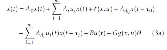where x ^∈ _Rⁿ, u ^∈ _R^m, θ ^∈ _R^q, y ^∈ _R^p are the states vector, the input control, the unknown parameters vector and the output vector, respectively. τ_i for i = 0,…,m are known constants delays. The matrices: A_i ∈ _R^n×n,

Adi ∈ Rn×n, for i = 0,…,m, B ∈ Rn×m, G ∈ Rn×r and C ∈ _R^p×n are known with constant values. The following assumptions are given and will be used in the sequel

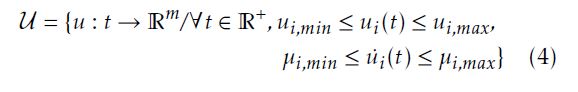
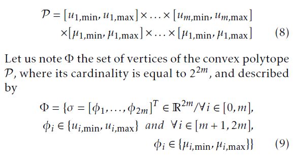
Assumption 1. The input u(t) is bounded such that u(t) ^{∈ U ⊂} _R^m, where

U = {u : t → Rm/∀t ∈ R+,ui,min ≤ ui(t) ≤ ui,max,

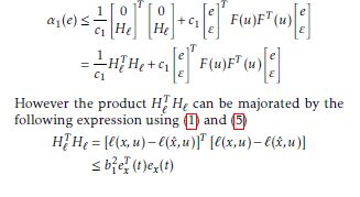
Assumption 2. The function `(x,u) : R^{n ×} _R^{m →} _Rⁿ is Lipschitz in x, ∀u ∈ U, i.e there exists a positive scalar b₁ such that

  ||`(x,u) − `(x^∗,u)|| ≤ b₁||x − x^∗||                 (5)

The function g(x,u) : R^{n ×} _R^{m →} _R^r×q is bounded ^∀x ^∈

Rn and ∀u ∈ U, that is there exists a scalar b_g such that

||g(x,u)|| ≤ b_g

and is Lipschitz in x, ∀u ∈ U, i.e there exists a positive scalar b₂ where

                     ||g(x,u) − g(x^∗,u)|| ≤ b₂||x − x^∗||                (6)

Assumption 3. The unknown parameters are supposed to be bounded such that there exists a scalar b₃ > 0 verifying

||θ|| ≤ b₃

Since assumption 1 holds, we have put the inputs u_i(t), for i = 1,…,m, and their derivatives in the same vector

In what follows, we point out the problem of the design of adaptive observer, which allows a simultaneous estimation of the states and the unknown parameters. As these observers are usually designed to be applied in robust and fault tolerant control, the add of the term Gg(x,u)θ in the system dynamics allows to model uncertainties affecting the system in the case of robust control, or may be used to model faults in the case of fault detection and isolation [18], [26], this term is more general than only the term Gθ as considered in [1] and in the section 3 of the present work.

In a first time, we propose an adaptive observer for system (3) without considering the presence of the nonlinear Lipschitz functions, i.e `(x,u) = 0 and g(x,u) = 1. In a second time, a more general adaptive observer is proposed for the considered class of nonlinear time delay systems (3). The obtained results do not lead to the results of the section before (see the discussion in section 5), which justify the structure of this work.

Before starting the observer design, let us give some useful relations used in this paper. For x ∈ _Rⁿ and y ∈ _Rⁿ, the following well known inequalities hold

2||x|| ||y|| ≤ βxxT +         yyT , ∀β > 0 β	(10)
xzT +zxT ≤ cxxT + 1zzT , ∀c > 0 c	(11)

3 Observer Design without Lipschitz nonlinearities

In this section, we consider system (3) without Lipschitz nonlinear functions, i.e. `(x,u) = 0 and g(x,u) = 1. Thus, an adaptive observer is proposed under the following form

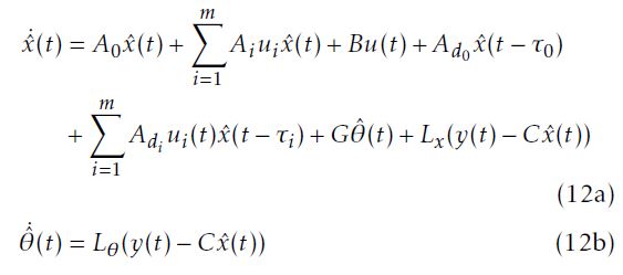
where xˆ(t) ∈ _Rⁿ and θˆ ∈ _R^q are the estimated states vector and the estimated unknown parameters vector, respectively. L_x ∈ _R^n×p and L_θ ∈ _R^q×p are the observer’s gains to be determined.

As a full order observer, we propose this structure of the observer, since it is the most commonly used in the literature, and had shown performance results. Within this observer, only two observer gains have to be determined, contrary to the full order observer structure as proposed in [23], which may be cumbersome to compute, due to the number of matrices to be computed.

The estimation error has the following dynamics

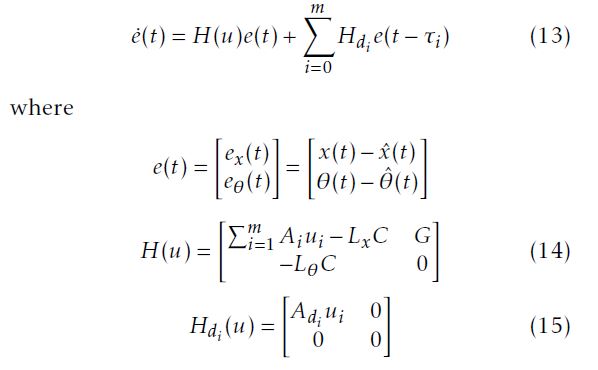
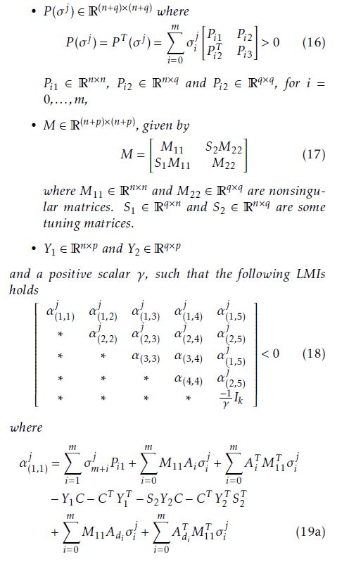
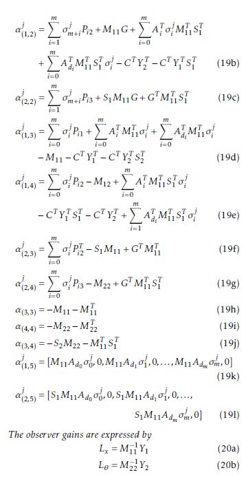
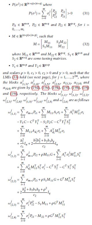
Theorem 1. Assume that assumption 1 holds. System (12) represents an adaptive observer to system (3) (with `(x,u) = 0 and g(x,u) = 1), and the estimation errors system (13) is quadratically stable for σ<sup>j</sup> ∈ Φ, j = 1,…,2<sup>2m</sup>, if there exist matricesNotice that we considered u<sub>0</sub>(t) = 1 for reasons of simplification. Then, system (12) is an adaptive observer for the delayed considered system described by (3) with `(x,u) = 0 and g(x,u) = 1, if and only if the estimation error system described by (13) is asymptotically stable. The stability of the estimation error e(t) and the computation of the observer’s gains L_x and L_θ are ensured via the following theorem.

 

Proof. The proof of the theorem 1 will be developed into two steps:

• In a first step, we give the stability conditionsusing a Lyapunov Krasovskii approach for LPV time delay systems, which leads to the resolution of an inequality.
• In a second step, we compute the observers ma-

trices and we transform the obtained inequality into LMIs, using a Polytopic approach.

First Step. Let us consider a Lyapunov Krasovskii function candidate with this form

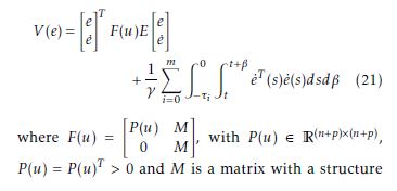
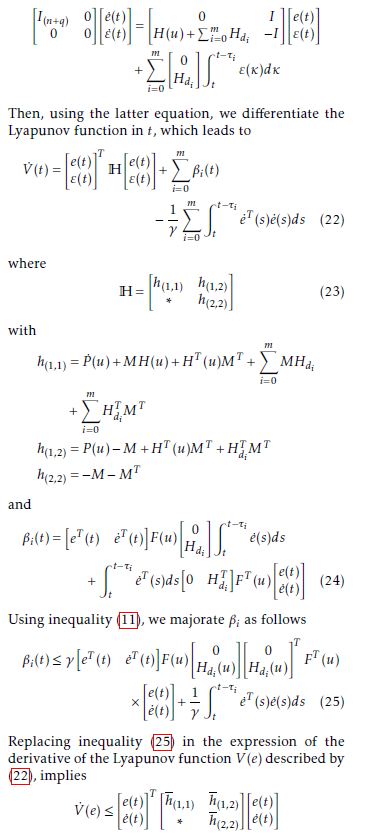
Let us note ε(t) = e˙(t), and we rewrite system (13) under a descriptor form as follows

       ”                #”        # ”                                       #”      #

         I(n0+q)    00   εe˙˙((tt)) = H(u)+P0 m_i=0Hdi         −II εe((tt))

Xm ” 0 #Z t−τ_i

+  ε(κ)dκ i=0 Hd_i t

Then, using the latter equation, we differentiate the Lyapunov function in t, which leads to

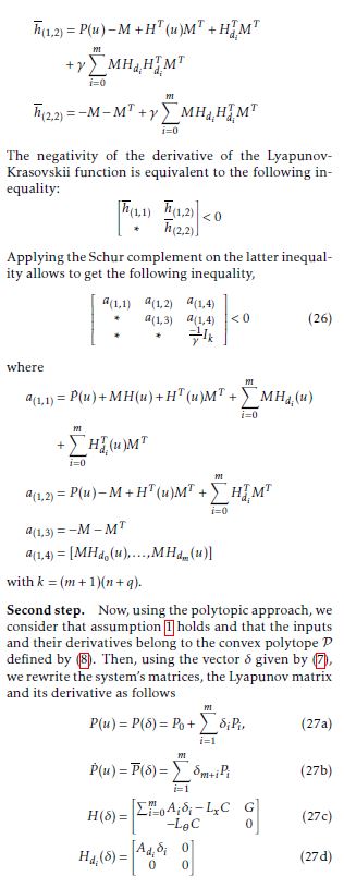
Then, we compute inequality (26) in the whole set of the vertices of the polytope Φ. By taking the matrices P ^j(σ_i) and M with the form (16) and (17) respectively, we obtain the results given in the proof, where the observer’s gains are given by (20).                                           0        0

Now, as discussed in the introductory section, we consider in the next section a more general class of systems with Lipschitz nonlinearities.

4 Observer Design with Lipschitz nonlinearities

In this section, the objective is to design an adaptive observer for system (3) with the following general structure in order to estimate simultaneously the states vector x and the unknown parameters θ. For that reason, the following adaptive observer is considered

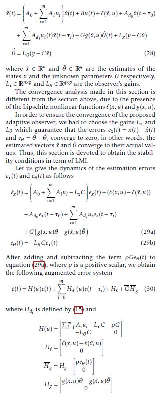
with u₀(t) = 1.

The quadratic stability of the estimation error system is ensured via the following theorem

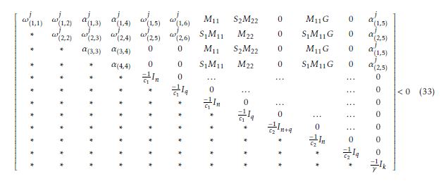
Theorem 2. Assuming that assumptions 1, 2 and 3 hold. System (28) is an adaptive observer for system (3), and the estimation error is quadratically stable for σ^j ∈ Φ, if there exist matrices

 

 

 

 

 

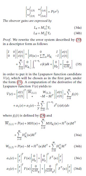
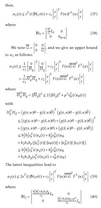
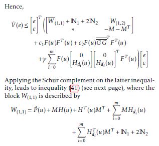
W₍₁,2), N1 and N2 are given by (36b), (38) and (40), respectively.

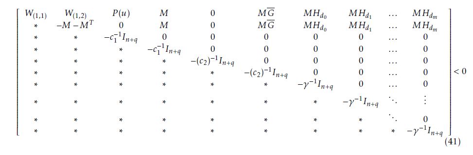
Finally, using notations (27) and the information on the inputs and their derivatives, we compute inequality (41), to extract the observer gains via LMIs, which completes the proof.

5         Discussion

1. In the literature, two major approaches have been developed to tackle the design of adaptive observer. These approaches are essentially based on:

(a) the elaboration of a parameter adaptation law. Here, the unknown parameter vector is deduced from the stability analysis of a state observer and the convergence property of the parameter error is obtained by a persistence of excitation type constraint. Many contributions deal with this approach as in [5], [15], [17], etc.

 

 

(b) an augmented system for which the adaptive observer design is elaborated. In this case, the system dynamics are augmented with the dynamics of its unknown parameters as in [20], [26], [27], [21].

In our work, the design of our adaptive observers are based on the approach described in item (b). However, those results are established by assuming a Lyapunov function where the derivative depends of both the state and parameters errors. So, the assumption of persistent excitation is not required in our work since the matrix appearing in the derivative of the Lyapunov function is not block diagonal, unlike in [15] where the boundedness of this derivative depends only of the state error terms.

2. The use of a descriptor approach and augmenting the estimation error system as done in the present work give more additional degrees of freedom to the problem resolution and allow to overcome the problem of the product between the Lyapunov matrix P (u) and the system’s dynamic matrix H(u) (see [28]).
3. First, due to the form of the block diagonalterms α_(3,3) and α_(4,4) appearing in both LMIs (18) and LMIs (33), the matrices M₁₁ and M₂₂ should be nonsingular matrices to satisfy the LMIs constraints. Notice that adding and subtracting the term ρGe_θ(t) from equation (29a) allow to have the matrix M₁₁ in the term ω_(2,2) in the LMI (33) given in theorem 2.

Second, the matrix M is chosen with the form given by (17) for the following reasons:

(a) If the matrix M is chosen under the following form

                                               ”                   #

                                        M = M11        M12

                                                 M21      M22

where M11 ∈ Rn×n and M22 ∈ Rq×q, M12 ∈ R^n×q and M₂₁ ∈ _R^q×n, we will come across the following problem

                                       ”        # ”         #

YY1121 ₌ MM1121 _Lx

(41)

                                       ”        # ”         #

YY1222 ₌ MM1222 _Lθ

Then, the existence of the observer’s gains depends on the following rank conditions

” # ” # rank M11 = rank M11 Y11

                                      M21                        M21      Y21

” # ” # rank M12 = rank M12 Y12

                                      M22                        M22      Y22

which add some non-convex constraints to satisfy in theorem 1 and 2.

(b) Putting the matrix M with a diagonal form, i.e. M₁₂ = 0 and M₂₁ = 0, implies that the blocks α_(2,2) and ω_(2,2) in LMIs (18) and (33) respectively, will be written as follow

m

                      j                  ^X j

α(2,2) =   σm+iPi3 i=1 m

                      j                X                     bg2 +b2b3bg +ρ2

                      ω(2,2) = i=1 σm+iPi3 ⁺  _c2   Iq

and one can see that the LMIs (18) and (33) can not be satisfied.

So, to avoid the above rank constraints, we set

M₂₁ = S₁M₁₁ and M₁₂ = S₂M₂₂ where matrices S₁ and S₂ are a priori chosen tuning parameters. This leads to Y₂₁ = S₁Y₁₁ and Y₁₂ = S₂Y₂₂.

However, one can see that, unlike matrix S₁, matrix S₂ does not appear in the diagonal blocks α_(2,2) and ω_(2,2) of LMIs (18) and (33), respectively. By the way, we can set S₂ = 0. Whereas, we need the condition S₁ , 0.

4. The obtained results in theorem 2 may appear as an extension of theorem 1. However, it is not the case. For the observer design in section 3, the nonlinear Lipschitz functions are taken as

`(x,u) = 0 and g(x,u) = 1

which imply that assumption 2 will be as follows

b₁ = 0, b₂ = 0 and b_g = 1

Applying this assumption on the results of theorem 2, do not lead to the results obtained in theorem 1, due to the fact that this assumption

j does not cancel some terms in the block ω_(2,2) of the LMIs (33). In addition, the bound b₃ of the unknown parameters θ is not required in the design of adaptive observer in section 3.

6 Numerical examples

To illustrate the efficiency and the feasibility of our results, we give in the sequel some numerical examples. Let us consider a bilinear time delay system, with

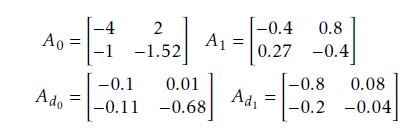
We assume that the system is controlled by one bounded input control u(t) = u₁(t)

−0.2 < u(t) = u₁(t) = 0.2sin(0.1t) < 0.2 with

” 0.8 #

B =

0.01

One can see, that the derivative is also bounded, such that

−0.02 < u˙(t) < 0.02

Then, we assume that the system is affected by one constant unknown parameters θ, where

“−0.09#

G =

0.9

The time delays are constant and known such that τ₀ = 0.9, and τ₁ = 0.4

The available measurement vector is given by

y(t) = x₁(t)

The Lipschitz nonlinear function g(x,u) is bounded and chosen as follows

−0.2 ≤ g(x,u) = 0.2sin(u(t) − x₁(t)) ≤ 0.2 and the function `(x,u) is given by

`(x,u) = “sin(x₂1((tt))ee−−00..22uu((tt))))# sin(x

The unknown parameters θ will be assumed to be bounded by b₃ = 0.5 only for the simulation in section 6.2.

6.1 Numerical results related to the first observer design without Lipschitz nonlinearities

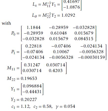
By computing the LMIs (18), given in theorem 1, in the set of the vertices of the convex polytope P, using the toolbox ”Lmilab”, we obtain the following matrices

 

 

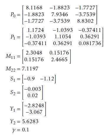
which yield to the following observer’s gains

−1 “−1.1484# L_x = M11 Y1 = −1.1728

L_θ = M₂₂⁻¹Y₂ = 0.79053

Figures 1, 2 and 3 show that the observer gives a suitable estimation of the states x₁ and x₂ and the unknown parameters θ. They prove also that even if the values of the unknown parameters change, but still constant, the estimation of the states and the unknown parameter converge to their real values.

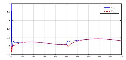Figure 1: Variation of the state x₁ (—) and its estimation xˆ₁ (· · ·).

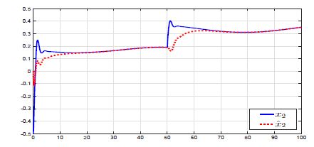Figure 2: Variation of the state x₂ (—) and its estimation xˆ₂ (· · ·).

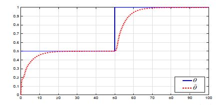Figure 3: Variation of the unknown parameter θ (—) and its estimation θˆ (· · ·).

6.2 Numerical results related to the second observer design with Lipschitz nonlinearities

By setting the tuning matrices S₁ and S₂ as follows

 Using the obtained gains into the observer yields to a suitable estimation of the states x(t) and the unknown parameter θ. The following figures show the effectiveness of our design.

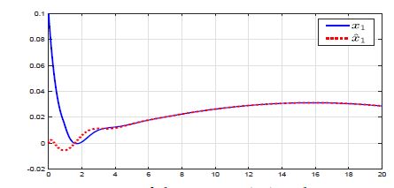Figure 4: Variation of the state x₁ (—) and its estimation xˆ₁ (· · ·).

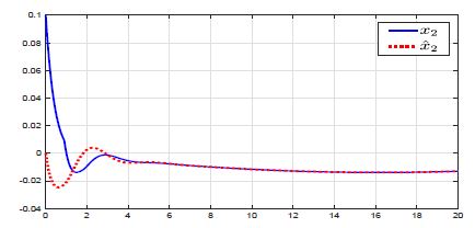Figure 5: Variation of the state x₂ (—) and its estimation xˆ₂ (· · ·).

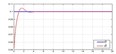Figure 6: Variation of the unknown parameter θ (—) and its estimation θˆ (· · ·).

7 Conclusion

The proposed adaptive observer for a class of nonlinear time delay system developed in this paper allows a suitable estimation of the state and the unknown parameter vectors, simultaneously. In a first time, a bilinear system with time delays is considered, which was extended by the addition of some nonlinear Lipshitz functions. The observer gains are obtained by solving LMIs in the vertices of a convex polytope. The simulation results show the performances and feasibility of the proposed approach. An extension of our adaptive observer design was presented in a second time, when a nonlinear Lipschitz functions interfere in the dynamics of a bilinear time delay system.

1. Sassi, H. Souley Ali, M. Zasadzinski, and K. Abderrahim, “Full order adaptive observer design for time delay bilinear system.” In the Proceedings of the 6th International Conference on Systems and Control, pp. 267–272, June 2017.
2. Bastin and M. Gevers, “Stable adaptive observers for nonlinear time-varying systems.” IEEE Transactions on Automatic Control, vol. 33, no. 7, pp. 650–658, 1988.
3. Besanc¸on, “Remarks on nonlinear adaptive observer design.” Systems and Control Letters, vol. 41, pp. 271–280, 2000.
4. Choi, H. Shim, Y. Son, and J. Seo, “Design of an adaptive observer for a class of nonlinear systems,” International Journal of Control, Automation and Systems, vol. 1, no. 1, pp. 28–34, 2003.
5. Ekramian, F. Sheikholeslam, S. Hosseinnia, and M. Yazdanpanah, “Adaptive state observer for Lipschitz nonlinear systems,” Systems and Control Letters, vol. 62, pp. 319–323, 2013.
6. Xie and P. Khargonekar, “Lyapunov-based adaptive state estimation for a class of nonlinear stochastic systems,” Automatica, vol. 48, pp. 1423–1431, 2012.
7. Zhao, X. Li, , and P. Li, “Adaptive observer design for a class of mimo nonlinear systems,” Proceedings of the 10thWold Congress on Intelligent Control and Automation, pp. 2198–2203, 2012.
8. Ibrir, W. Xie, and M. C. Su, “Observer-based control of discrete-time Lipschitizian nonlinear systems: Application to one-link flexible joint robot.” International Journal of Control, vol. 78, no. 6, pp. 385–395, 2005.
9. Zemouche and M. Boutayeb, “On LMI conditions to design observers for Lipschitz nonlinear systems.” Automatica, vol. 49, pp. 585–591, 2013.
10. Richard, “Time-delay systems : An overview of some recent advances and open problems,” Automatica, vol. 39, no. 10, pp. 1667–1694, 2003.
11. Kadhraoui, M. Ezzine, H. Messaoud, and M. Darouach, “Design of unknown input functional observers for delayed singular systems with state variable time delay,” Transactions on Systems and Control, vol. 10, pp. 503–509, 2015.
12. Briat, O. Sename, and J. Lafay, “Design of LPV observers for LPV time-delay systems: an algebraic approach.” International Journal of Control, vol. 84, no. 9, pp. 1533–1542, 2011.
13. Fridman, “Tutorial on Lyapunov-based methods for timedelay systems,” European Journal of Control, vol. 20, pp. 271– 283, 2014.
14. Gu, V. Kharitonov, and J. Chen, Stability of Time-Delay Systems. Birkh¨auser Boston, 2003.
15. Cho and R. Rajamani, “A systematic approach to adaptive observer synthesis for nonlinear systems,” IEEE Transactions on Automatic Control, vol. 42, no. 4, pp. 534–537, 1997.
16. Wang, Y. Dong, and W. Qin, “Adaptive observer design for a class of Lipschitz nonlinear systems,” In the proceedings of the 30th Chinese Control Conference, pp. 665–669, July 2011.
17. Pourgholi and V. Majd, “Robust adaptive observers design for lipschitz class of nonlinear systems.” International Journal of Electrical and Computer Engineering, vol. 6, no. 3, pp. 275– 279, 2012.
18. Zhang and B. Deylon, “A new approach to adaptive observer design for mimo systems,” American Control Conference, vol. 2, pp. 1545 – 1550, 2001.
19. Besanc¸on, J. D. Le´on-Morales, and O. Huerta-Guevara, “On adaptive observers for state affine systems.” International Journal of Control, vol. 79, no. 6, pp. 581 – 591, 2010.
20. Alma and M. Darouach, “Adaptive observer design for a class of linear descriptor systems.” Automatica, vol. 50, pp. 578–583, 2014.
21. Farza, I. Bouraoui, T. M´enard, and R. Ben Abdennour, “Adaptive observer for a class of uniformly observable systems with nonlinear parametrization and sampled outputs.” Automatica, vol. 50, pp. 2951–2960, 2014.
22. Alma, H. S. Ali, M. Darouach, and N. Gao, “An H1 adaptive observer design for linear descriptor systems.” 2015 American Control Conference, pp. 4838–4843, May 2015.
23. Sassi, H. Souley Ali, S. Bedoui, K. Abderrahim, and M. Zasadzinski, “Design of a functional adaptive observer for bilinear delayed systems.” 13th IFAC workshop on Time Delay Systems TDS, vol. 49, no. 10, pp. 25–30, 2016.
24. Sassi, M. Zasadzinski, H. Souley Ali, and K. Abderrahim, “Design of an H-infinity adaptive observer for bilinear delayed systems.” The 20th World Congress of the International Federation of Automatic Control (IFAC WC), vol. 50, no. 1, pp. 2923–2928, July 2017.
25. Khalil, Nonlinear Systems, Third Edition. USA: Prentice Hall, 2002.
26. Zhang, “Revisiting different adaptive observers through a unified formulation.” Proceedings of the 44th IEEE Conference on Decision and Control, and the European Control Conference., pp. 3067–3072, December 2005.
27. Ahmed Ali, R. Postoyan, and F. Lamnahbi Lagarrigue, “Continuous-discrete adaptive observers for state affine systems.” Automatica, vol. 45, pp. 2986–2990, 2009.
28. G´erard, H. Souley Ali, M. Zasadzinski, and M. Darouach, “H-infinity filter for bilinear systems using LPV approach,” IEEE Transactions on Automatic Control, vol. 55, no. 7, pp. 1668–1674, 2010.

(Click to view)

(Click to view)