1. Introduction

This paper is an extension of work originally presented in the 48th European Microwave Week [1] where a four layer’s wideband (6 – 18 GHz) meander-line polarizer has been optimized and simulated with different patch antenna for validation.

As well known, the polarizer is a passive broadband device, used to change the polarization properties of an Electro-Magnetic (EM) wave. Combining antennas with those devices to change the polarization of the wave is very useful. A well-designed polarizer permits to change the antenna polarization and to propagate a different polarization without any significant variations in the pattern performance [2]. The Meander-Line (ML) polarizer is the most popular device used to change the Linear Polarized (LP) waves into the Circular Polarized (CP) ones [3]. It is a multilayer structure made of several printed ML sheets spaced by about one-quarter wavelength apart. The principle of operation is to convert an incident wave into two equal components at ±45⁰ as summarized in [4]. One component passes through a structure equivalent to a broad-band shunt-inductive filter while the other passes through a broad-band shunt-capacitive filter. the other component, by about 45⁰.

The ML polarizer has been proposed in [4], and improved in [5]. Later, [6-9] gave analytical formulas to compute the phase delay and characterize the polarizer’s grating layer. Transmission Line (TL) theory together with Method of Moments (MOM) based algorithms has been used by [7, 10-13] to analyze the ML polarizer.

In this paper, the basic principle of the ML polarizer is described in section 2. Section 3 describes the detail of the optimization procedure which includes the TL equivalent circuit and Simulated Annealing (SA) algorithm. Finally, in section 4, the four layer’s wideband (6 – 18 GHz) meander-line polarizer studied previously in [1] is used as a case study. The optimization study is presented, followed by experimental validation using a wideband horn antenna covering the same bandwidth.

2. Meander Line Polarizer: Basic Principle

The ML polarizer is a multilayer structure (Figure 1). Each layer consists of MLs printed on a low-loss dielectric substrate and separated by a spacer respecting one-quarter wavelength apart. The spacer could be air (vacuum) or any kind of low loss material such as foam or dielectric substrate.

The principle of operation is to convert an incident wave into two equal and perpendicular components at ±45 degrees as summarized in [3]. The ML polarizer’s layer is placed in the xy-plane in such a way that the meander axes are all oriented at an angle Ψ = 45 degrees with respect to the incident electric field  along the y-axis (Figure 2).

The incident electric field  will be decomposed into two orthogonal components: one parallel and the other one perpendicular to the ML axis, noted respectively  and . As well known, a CP wave can be obtained by designing a ML polarizer that introduces a differential phase shift of 90⁰ between the components and  while keeping their magnitudes identical over the entire required frequency bandwidth. Right-hand or left-hand circular polarizations can be easily obtained by switching the orientation angle Ψ from +45⁰ to -45⁰.

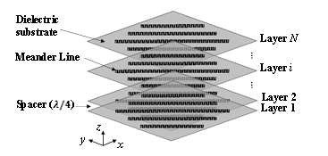Figure 1: N-Layers ML polarizer design

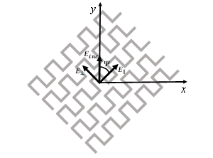Figure 2:  Incident field ( ) exiting the polarizer layers with the parallel and the perpendicular  components resulted.

The difficulty in the design of a meander-line polarizer is to determine the inductive and capacitive impedances of the grating for the and  polarizations with respect to frequency and constitutive dimensions of the meander line.

An optimization method is developed to optimize the ML polarizer’s dimensions and described in detail in the below section. It consists of a semi-analytical analysis based on the combination of TL circuit theory and SA algorithm and allows to find the dimensions of the MLs that keep the magnitude of the components and  identical with a  phase differential shift of 90⁰ over the desired frequency bandwidth.

Our method of optimization has the advantage of avoiding the heavy computations and simulations used in [13] to solve the TL circuit and the unit cell of each layer. This implies a large reduction in the computation time.

• The TL equivalent circuit is solved using the optimization tool of ADS. This tool has the advantage of optimizing the shunt elements of all the layers at one simulation and avoid the heavy computation of the transmission matrices of each layer then the scattering transmission parameters and finally optimize the shunt elements using quasi-Newton algorithm as used in [13].
• SA algorithm is used to optimize the physical dimensions of the MLs. This algorithm optimizes the dimensions and minimize the absolute values of the differences between the theoretical admittances introduced by Chu and Lee in [14], and their lumped-element counterparts optimized by solving the TL circuit using the optimization tool of ADS. This method avoids the full-wave analysis of the unit cell and all the steps described before which are used in [13].

3. Meander Line Polarizer: Optimization and validation Procedures

3.1.  TL Equivalent Circuit Model

As summarized in [4], the incident electric field  will be  decomposed into two orthogonal components and . One component passes through a structure equivalent to a broad-band shunt-inductive filter while the other passes through a broad-band shunt-capacitive filter. The phase shift through either filter should have almost the same slope, so that if the differential phase shift is 90⁰ at one frequency in the common passband, it remains close to 90⁰ everywhere in the common passband.

The TL equivalent circuit of the N-layers ML polarizer excited by an incident wave along y-axis (Figure 1) can be represented as shown in the Figure 3 where ?₀ is the characteristic impedance of the vacuum ( ) with  and  the permeability and the permittivity of vacuum, respectively. The parameters
h_d1, h_d2, …, h_dN and , , …,  are respectively the thickness and the relative permittivity of the 1^st, 2^nd, …, N^th layer. The parameters h_s1, h_s2, …, h_sN and , , …,  are respectively, the thickness and the relative permittivity of the
1^st, 2^nd, …, N^th separator. The , , …,   and
, , … ,  are respectively, the lumped inductance and capacitance equivalents of the 1^st, 2^nd, …, N^th periodic strip lines on each layer.

The input parameters of the TL model of ML polarized are:  the frequency bandwidth (center frequency f₀), the number of layers and the relative permittivity and thickness of each dielectric substrate and separator. This model must be solved by
optimizing the shunt components , , …,  and
, , …,  which verify the maximum transmission coefficients (S₂₁ and S₄₃) in term of magnitude (~0dB) while attaining 90⁰ differential phase shift between both components for the CP properties.

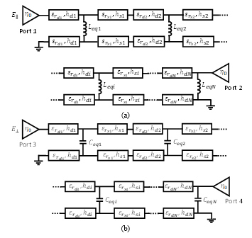Figure 3: Transmission Line equivalent circuit for N-Layers ML polarizer observed by (a) the parallel wave  and (b) the perpendicular wave .

3.2.  Simulated Annealing Algorithm

Simulated Annealing is a mathematical equivalent of the thermodynamic annealing. The energy of the particle in thermodynamic annealing process can be compared with the cost function to be minimized in optimization problem. The particles of the solid can be compared with the independent variables used in the minimization function. The Simulated Annealing Algorithm is detailed in [15].

The MLs dimensions must be optimized to verify that the impedance equivalent of each layer is equal to the one found by solving the TL circuit model.

Chu and Lee in [14], presented rigorous empirical formulas of equivalent admittances for parallel ( ) polarization  and perpendicular ( ) polarization  of the ML, dependent on the dimensions a, b, h, and w (Figure 4).

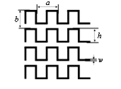Figure 4: Polarizer’s dimensions

The SA algorithm is used to optimize the best values of the ML dimensions of each layer i by making the admittances values (  and ), found using the TL circuit model, equal to the ones given by Chu and Lee (  and ). In other word, for each layer i, the dimensions  are optimized to minimize the difference between the admittances (  and ) as shown in the equation (1).

The optimization procedure is summarized in Figure 5.

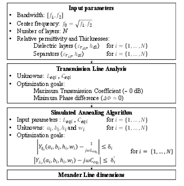Figure 5: Optimization Procedure Summary

4. Case Study: 6-18GHz Four Layers ML Polarizer

A four layers ML polarizer covering the bandwidth from
6 GHz to 18 GHz is studied in this section.

4.1.  Polarizer Optimization

The optimization procedure starts by defining the input parameters which are the frequency bandwidth [6-18GHz], center frequency f₀ = 10.4GHz, number of layers N = 4, relative permittivity and thickness of the dielectric substrates ( , h_di) and separators ( , h_si)  for .

To simplify the TL equivalent model, the equivalent circuit was studied with one-quarter wavelength apart ( ) air separators and without considering the substrate effect since a very thin substrate ( ) with low permittivity and low loss (Rogers RT/duroid 5880 ( , )) is used.

The choice to have the same MLs dimensions (i.e. same L_eq and C_eq) for each layer was also made to make the system integration simple and flexible. The TL equivalent circuit of the four layers ML polarizer is shown in the Figure 6.

The optimization tool of ADS is used to find the best values of the equivalent inductance and capacitance to verify the maximum transmission coefficients (S₂₁ and S₄₃) in term of magnitude (~ 0dB) and 90⁰ differential phase shift between them over the entire bandwidth. The optimum values are: =3 fF and  = 0.494 pH.

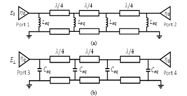Figure 6: TL circuit model of the four layers Meander Line polarizer observed by the (a) parallel wave ( ) and the (b) perpendicular wave ( ).

The ML dimensions (a, b, h, and w) are optimized using the SA algorithm, as detailed previously, by making the admittances values (  and ), found using the TL circuit model (Figure 6), as close as possible to the ones given by Chu and Lee (1). The optimum values found are a = 2.17mm, b = 13.08mm,
w = 0.446mm and h = 5.151mm.

4.2.  Polarizer test with 6-18GHz Horn Antenna

To verify the performance of ML polarizer, a wideband horn antenna (6 to 18 GHz) shown in figure 7(a) is used. The four ML layers of the polarizer were fabricated. A mechanical support was designed and realized using a 3D printer to maintain the quarter wave length distance between each layers and the antenna. The picture of the polarizer attached to the antenna is shown in
figure 7(b). Figure 7(c) shows the antenna with the ML polarizer under test in the near field anechoic chamber StarLab (by Microwave Vison Group), available in IETR.

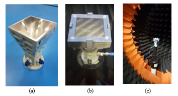Figure 7: Picture of (a) horn alone – (b) horn with ML-Polarizer – (c) horn with ML-Polarizer under test

The measurements were performed for the horn antenna alone and with the ML polarizer excited in vertical polarization. The reflection coefficients of the horn antenna alone (without the ML polarizer) and with the ML polarizer are plotted in Figure 8.

Both reflection coefficients are very close, which proves that the ML polarizer doesn’t mismatch the antenna except at the around 6GHz, where the reflection coefficient is measured around -6.5dB.

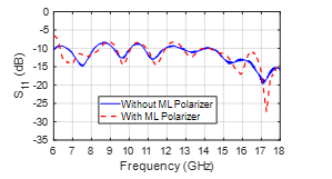Figure 8: Reflection coefficients of the horn antenna with and without the ML polarizer

The co-polarization and cross-polarization of the Electrical filed (  and ) are plotted for different frequencies in the figures 9-15.

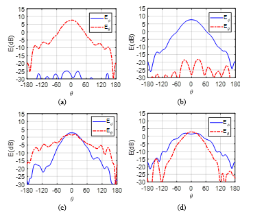Figure 9: Measured  and  at 6 GHz for the horn antenna alone in both planes (a)  and (b)  and for the horn antenna with the ML polarizer in both planes (c)  and (d) .

In figure 9, the  and  components of horn antenna alone and with ML polarizer are plotted at 6 GHz in both planes (  and ). The results seem to show that the horn antenna initially excited for a vertical polarization (Figure 9 (a) and (b)) is radiating a circular polarized wave when it is stacked with the ML polarizer (Figure 9 (c) and (d)). At the boresight, the difference between the co and cross components of the horn antenna measured alone is more than 28 dB while it reduces to 1dB when the horn antenna is measured with the ML polarizer. The measured Axial Ratio (AR) of the horn antenna with the ML polarizer at this frequency is around 6dB (Figure 16). Therefore, the ML polarizer is converting the linear polarization waves into elliptical polarized ones. The measured insertion losses are around 2.5dB (Figure 17) which is due to the mismatch of the antenna with the ML polarizer at this frequency (Figure 8).

The  and  components of the horn antenna alone and with ML polarizer are plotted in figure 10 – 14 for the frequencies from 8GHz to 16GHz.  The vertical polarized waves of the horn antenna alone are perfectly converted to circularly polarized ones when it is stacked to the ML polarizer with the maximum AR of 2.9 dB at 8GHz (Figure 16).  The insertion losses are less than 1.4 dB with the minimum of 0.24 dB at 14 GHz (Figure 17).

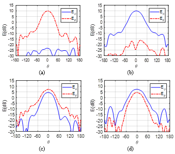Figure 10: Measured  and  at 8 GHz for the horn antenna alone in both planes (a)  and (b)  and for the horn antenna with the ML polarizer in both planes (c)  and (d) .

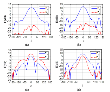Figure 11: Measured  and  at 10 GHz for the horn antenna alone in both planes (a)  and (b)  and for the horn antenna with the ML polarizer in both planes (c)  and (d) .

The measured results at 18 GHz are plotted in figure 15. At the plane , some ripples are observed in the pattern of the co-component when the antenna is measured with the ML polarizer. This comportment is not reproduced at the other cut plane ( ) where the directive radiation pattern shape is preserved. The measured Axial Ratio (AR) of the horn antenna with the ML polarizer at this frequency is around 5.4 dB (Figure 16). Therefore, the linearly polarized waves of the horn antenna alone are converted to elliptical polarized waves. The measured insertion losses are around 0.6 dB (Figure 17).

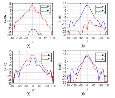Figure 12: Measured  and  at 12 GHz for the horn antenna alone in both planes (a)  and (b)  and for the horn antenna with the ML polarizer in both planes (c)  and (d) .

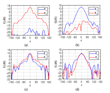Figure 13: Measured  and  at 14 GHz for the horn antenna alone in both planes (a)  and (b)  and for the horn antenna with the ML polarizer in both planes (c)  and (d) .

The measured values of the AR at boresight are reported in figure 16 versus frequency for the horn antenna with the ML polarizer. The AR is less than 3dB at the frequency band between 8 GHz and 16 GHz. Therefore, the ML polarizer converts the linear polarization of the horn antenna to a circular one. In both ends of the frequency band (6 GHz and 18 GHz), the ML polarizer converts the linear polarization of the horn antenna to an elliptical one.

The total electrical fields (E_tot) values at boresight are reported in figure 17 versus frequency for the horn antenna alone and with the ML polarizer. This figure shows clearly that the E_tot of the horn antenna with the ML polarizer is following the same allure as the E_tot of the horn antenna alone variation with some insertion losses.

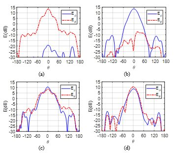Figure 14: Measured  and  at 16 GHz for the horn antenna alone in both planes (a)  and (b)  and for the horn antenna with the ML polarizer in both planes (c)  and (d) .

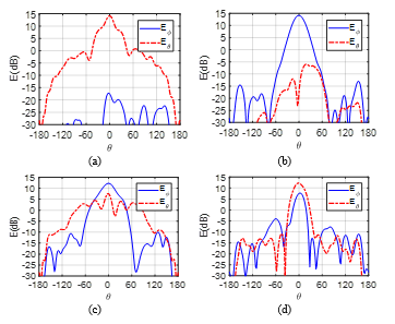Figure 15: Measured  and  at 18 GHz for the horn antenna alone in both planes (a)  and (b)  and for the horn antenna with the ML polarizer in both planes (c)  and (d) .

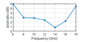Figure 16: Measured Axial Ratio (AR) versus frequency for the horn antenna with the ML polarizer

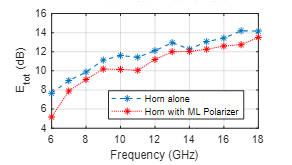Figure 17: Measured total electrical field (E_tot) versus frequency for the horn antenna alone and with the ML polarizer

In almost the entire bandwidth, except at 6 GHz, the insertion losses are less than 1.5dB with the minimum of 0.24 dB at 14 GHz. The maximum insertion losses (2.5dB) are measured at 6 GHz which is due to the mismatch of the horn antenna with the ML polarizer.

5. Conclusion

An optimization Method of Wideband Multilayer Meander-Line Polarizer using a Semi-Analytical approach is described in this paper. The originality of this method lies in the optimization of: i) values ​​of the shunt equivalent inductance L_eq and capacitance C_eq, determined by the ADS software – ii) ML dimensions (a, b, h and W) using the SA algorithm. This method was applied to optimize a four layers wideband (6 – 18 GHz) ML polarizer as study case.

The optimized polarizer was manufactured and a wideband Horn antenna covering the same bandwidth was used for the testing. The test consists of the measurements of the horn antenna vertically polarized without and with the ML polarizer. Good measured results were observed where the linear polarization of the antenna was converted to a purely circular one in almost the entire frequency band (8 GHz – 16 GHz, corresponding to an octave). In both ends of the frequency band (6 GHz and 18 GHz), an elliptical polarization was achieved with a maximum axial ration of around 6dB.

At 6GHz, the axial ratio is around 1dB but the insertion losses are around 2.5dB which is due to the mismatch of the horn antenna with the ML polarizer at this frequency.  At 18 GHz, the axial ratio is around 5dB and the insertion losses are around 0.6 dB.

 The future work will be devoted to the study of five layers ML polarizer to improve the performances, and especially at both ends of the frequency band.

1. W. Abdouni, M. S. Khan, A. Konstantinidis “Design of a Wideband Multilayer Meander-Line Polarizer (6 – 18 GHz) using a Semi-Analytical Method,” in 48th European Microwave Conference (EuMC), Madrid Spain, 2018, https://doi.org/10.23919/EuMC.2018.8541675
2.  R. A. Marino, “Accurate and efficient modeling of meanderline polarizers,” Microw. J., 41 (11), 22-34, Nov. 1998
3.  J. F. Zurcher, “A meander-line polarizer covering the full E-band (60-90 GHz),” Microwave Opt. Technol. Lett., 18, 320-323, Aug. 1998. https://doi.org/10.1002/%28SICI%291098-2760%2819980805%2918%3A5<320%3A%3AAID-MOP3>3.0.CO%3B2-A
4.  L. Young, L.A. Robinson, and C.A. Hacking “Meander-Line Polarizer,” IEEE Transactions on Antennas and Propagation, 21(3), 376-378, 1973. https://doi.org/10.1109/TAP.1973.1140503
5.  J. J. Epis, “Broadband antenna polarizers,” US Patent 3754271, Aug. 1973.
6.  T. L. Blackney, J. R. Burnett, and S. B. Cohn, “A design method for meander-line circular polarizers,” 22nd Ann. Antenna Symp., 1-5, Oct. 1972.
7.  C. Terret, J. R. Level, and K. Mahdjoubi, “Susceptance computation of a meander-line polarizer layer,” IEEE Transactions on Antennas and Propagation, 21, 1007-1011, Sep. 1984. https://doi.org/10.1109/TAP.1984.1143456
8.  S. W. Lee, and G. Zarrilo, “Simple formulas for transmission through periodic metal grids or plates,” Antenna Application Sym., University of Illinois, Urbana, IL, Sponsored by RADC (EEA) Electromagnetic Sciences Division, Hanscom AFB, 1983. https://doi.org/10.1109/TAP.1982.1142923
9.  A. K. Bhattacharyya, and T. J. Chwalek, “Analysis of multilayered meander line polarizer,” Int. J. of Microwave and Millimeter-wave Computer-aided Eng., 442-454, 1997. https://doi.org/10.1002/(SICI)1522-6301(199711)7:6%3C442::AID-MMCE6%3E3.0.CO;2-P
10.  M. A. Joyal, and J.-J. Laurin, “Analysis and design of thin circular polarizers based on meander lines,” IEEE Transactions on Antennas and Propagation, 60, 3007-3011, Sep. 2012. https://doi.org/10.1109/TAP.2012.2194659
11.  C. C. Chen, “scattering by a two-dimensional periodic array of conducting plates,” IEEE Transactions on Antennas and Propagation, 18, 660-665, 1970. https://doi.org/10.1109/TAP.1970.1139760
12.  R. S. Chu, and K. M. Lee, “Radiation impedance of a dipole printed on periodic dielectric slabs protruding over a ground plane in an infinite phased array,” IEEE Transactions on Antennas and Propagation, 35, 13-25, 1987. https://doi.org/10.1109/TAP.1987.1143966
13.  M. Letizia, B. Fuchs, C. Zorraquino, J.-F. Zurcher, and J. R. Mosig, “Oblique incidence design of meander-line polarizers for dielectric lens antennas,” Progress In Electromagnetics Research B, 45, 309- 335, 2012. https://doi.org/10.2528/PIERB12080807
14.  RUEY-SHI CHU, KUAN-“I LEE, “Analytical Model of a Multilayered Meander-Line Polarizer Plate with Normal and Oblique Plane-Wave Incidence,” IEEE Transactions on Antennas and Propagation, 35(6), 652 – 661, 1987. https://doi.org/1987 10.1109/TAP.1987.1144158
15.  E.S. Gopi, “Algorithm Collections for Digital Signal Processing Applications Using Matlab”, Mathematics\\Wavelets and signal processing, 2007.

(Click Here)

(Click Here)