1.Introduction

The time series forecasting problem is an attractive and vital research issue. This forecasting problem has been often handled by using a variety of methods like mathematical statistics, artificial neural networks, etc. The downsides of the traditional time series forecasting models are that they extensively dependent on historical data or require having the linearity assumption and cannot solve prediction problems in which the values of time series are linguistic terms. To overcome these difficulties, the authors in [1, 2] first produced the concepts of FTS, which have the ability to deal with vague and incomplete data sets by utilizing the fuzzy set theory [3]. They have proposed the two FTS forecasting models to implement on university enrolments of Alabama with a forecasting schema consisting of main five steps: (1) defining UoD, (2) Partitioning of the UoD into intervals, (3) determining the fuzzy sets and fuzzifying the time series, (4) Establishing fuzzy logical relationship, and (5) forecasting and defuzzifying the forecasting values.
However, their approaches take a lot of time to build forecasting model because of using the complex max– min operations in fuzzy relationship matrix and lack of persuasiveness in partitioning the UoD. These limitations led research [3] to develop a new FTS forecasting model using simple arithmetic operations to replace the complex matrix operations [1, 2] in the determination of fuzzy relationship matrix and defuzzification output values. In addition, research works [5, 6] found out the importance of assigning weights to deal with the issue of recurrent fuzzy relationship and to reflect the difference in their importance. Expansion of the framework [3] into a high-order FTS schema [7], and the influence of the length of intervals in article [8] come with the development from the one-factor FTS models into two-factor FTS model [9]. These forecasted approaches are the basis for the strong development of many FTS models in the next time periods. Recently, many authors have applied different advanced data mining techniques in each stage of FTS model with view to enhancing forecasting accuracy. Study in article [10] used the automatic clustering technique for partitioning the UoD into unequal – size intervals at the fuzzification stage in their forecasting model. Some other researches apply soft computing techniques(especially evolutionary computing, clustering techniques) for adjusting and selecting intervals with unequal-size, can be found as genetic algorithm [11, 12], simulated annealing [13], PSO [14-22], K-mean [23, 24], fuzzy C-means [25, 26]. Just recently, a completely different way from fuzzy approach, several works with regards to HA have been published. In [27], the authors have presented a forecasting method based on the theory of hedge algebra [28] for forecasting university enrolments, to be a typical option. In which, the hedge algebra was used to construct linguistic domains and variables instead of performing data fuzzification and defuzzification in the fuzzy approach. In addition, researches in [29, 30] proposed the HA-based forecasting models to obtain unequal – length intervals in the UoD by mapping the semantics of linguistic variables into fuzziness intervals. However, two these research works only focus on building the first-order forecasting model to apply the number of students annually at the University of Alabama. In addition, their forecasting models have not yet applied the optimal techniques, so the obtained forecasting results are not really good enough.
Based on analyzing of the aforementioned research works showed that determining of the length of interval and the order of fuzzy relationships affect strongly forecasting performance of the model. To avoid the above – mentioned limitations and promote the advantage of combination with methods of partitioning in the UoD. The purpose of this study is to suggest a new partition method which uses PSO algorithm to optimize parameters of HA in the FTS prediction model. Therefore, we develop a novel hybrid prediction model using method of fuzzy relation group [17], integrating with HA and PSO algorithm in the identification of optimal intervals with view to enhancing the forecasting performance of the proposed model. For making it become reality, HA has been used to divide the UoD into intervals with unequal – size based on the parameters optimized by PSO. After obtaining the intervals, the time series data is put into the intervals by fuzzy sets and used them to create the FLRs, group of FLRs. Later, all information in FLR groups are utilized to produce the final prediction results based on the our defuzzification principle [31]. Finally, to enhance the accuracy of the model, we continue applying PSO algorithm to readjust the initial interval lengths which are obtained by fuzzy parameters of HA into intervals with the more proper length. Our forecasting model is examined on two following real-world datasets: 1) the historical enrolment dataset of University of Alabama [3], 2) the dataset of car road accident [32]. The examined results point out that our forecasting model outperforms the some of the recent FTS models in terms of prediction accuracy rate.
The next content of this paper introduces brief fundamental theories related to FTS model such as, fuzzy time series, Hedge Algebras and PSO algorithm. A method using PSO technique which has never been applied before in the selecting optimal parameters of HA and optimal length of intervals simultaneously, is presented in Section 3. Section 4 discusses the forecasting performance by comparing the obtained results of the proposed model with ones of the previous models. The last section gives conclusions and directions for future work.
The Fundamental Theories and Algorithms
In this section, we briefly introduce general knowledge related to FTS which is proposed in [1, 2] and improved by study [3]. In addition to, the hedge algebras [28] and PSO algorithm [33] is also reviewed.
Fuzzy time series
The concepts of FTS were proposed in [1, 2], in which the historical time series data are given in the form of fuzzy sets [3].
Assume that Y(t) (t = ..,0,1,2 ..) a real subset R (Y(t)  R), regarded as the UoD on which the fuzzy sets f_i (t) (i = 1,2…) are defined. If F(t) including the collection of f_1 (t),f_2 (t),… , then F(t) is namely a FTS which is defined on Y(t) [1, 2]
If there exists fuzzy logical relationship (FLR) between F(t-1) and F(t), namely R(t-1, t), such that they can be expressed as F(t) = F(t-1) R(t-1, t) or F(t-1)→ F(t) ; Where R(t-1, t) is the first- order fuzzy relationship between F(t) and F(t-1) and “ ” represents the max–min composition operator. Here F(t) and F(t-1) are fuzzy sets. If, let Ai = F(t) and Aj = F(t-1), the relationship between F(t) and F(t -1) is replaced by Ai → Aj , where Ai and Aj are called the current state and the next state of fuzzy relationship, respectively [1, 2, 4]
Let F(t) be a fuzzy time series. If F(t) is derived by more fuzzy sets F(t-1), F(t-2),…, F(t-β+1), F(t- β), then fuzzy relationship between them can be represented as F(t- β), …, F(t-2), F(t-1) → F(t). This relationship is called the β – order FTS model [1, 2, 7]
Suppose that F(t) is derived from F(t-1), then the relationship can be denoted as F(t-1)→ F(t). If, let 〖 A〗_i (t) = F(t) and A_j (t-1)= F(t-1). The FLR of them can be replaced as A_j (t-1)→ A_i (t). In addition, at the time t, there are also exists fuzzy relationships as 〖 A〗_j (t1-1)→ A_i1 (t1),..,A_j (tn-1)→ A_in (tn) with t1,t2,..,tn≤ t. It is noted that Ai(t1), Ai (t2),…, and Ai(tn) having the same fuzzy set Ai, but look at different times t1, t2,…, and tn, respectively. If these FLRs appear before A_j (t-1)→ A_i (t), they can be grouped into a fuzzy relationship group as follows: A_j (t-1)→ A_i1 (t1) 〖,A〗_i2 (t2),〖…,A〗_in (tn),A_i (t), and it is called TV-FRG [17].
Some basis concepts of Hedge Algebras
Hedge Algebras are introduced by N.C. Ho in 1990. It is considered as a new approach to solve forecasting problems in which it is used to quantify the linguistic variables. Each of linguistic variable X is represented by an algebraic structure, which is built on the inherent semantic order of the linguistic terms [28] and defined as follows:
Definition 1: The linguistic variable X is a set including 5 components AX=(X,G,C,H,≤) and called HA;
In which, X is the basic set in AX; “ ≤ ” is a natural semantically ordering relation on X; G={c^-,c^+ }, c^-≤c^+ is the set of generating elements (eg., Low ≤ High) ; C = {0, w, 1} is a set of constants, with (0≤c^-≤ W≤c^+≤1); H=H^-∪H^+, with H^-={ h_(i ): -q≥i≥ -1} denotes the set of all negative hedges of X, and H^+={h_i:1≤i≤p} denotes the set of all positive hedges;
Definition 2. Let AX = (X, G, C, H, ) be a HA. The function fm: X→[0,1] is named to be a fuzziness measure of elements in X, if:
1) fm(c^- )+fm(c^+ )=1 and ∑_(h∈H)▒〖fm(hx)=fm(x) 〗 with ∀x∈X;
2) f(x) = 0 with ∀xϵX so that fm(0)=fm(W)=fm(1)=0
3) For ∀x,y∈X,∀h∈H, fm(hx)/fm(x) =fm(hy)/fm(y) , this equation does not depend on x; y and it is called fuzziness measure of the hedge h and namely by (h). The properties of fm(x) and (h) are given as below:
Proposition 1. The fm denotes the fuzziness measurement on X, the following statements hold.

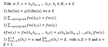
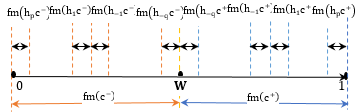Figure 1: The order of fuzziness measure of elements x∈X,h_j∈H,c∈G.

Particle swarm optimization
PSO is an evolutionary computation algorithm which is introduced by article [33] for searching the global optimum solution. It is developed by work [14] for applying in the forecasting field. Each particle in the swarm represents a potential solution to the global optimization problem. When particles move from this position to other position in q-dimensional space, all particles (i.e, N particles) have fitness values which are estimated according to fitness function. In the moving process of particles. The position of the best particle among all particles found so far is saved and each particle maintains its individual best position which has passed previously. Each individual particle kd (1≤ kd ≤ N) is composed of three components: its position P_kd=[p_(kd,1),p_(kd,2),…,p_(kd,q)], the velocity vector V_kd=[v_(kd,1),v_(kd,2),…,v_(kd,q)] and the best position that it has individually found so far P_(best,kd)=[ P_(kd,1),P_(kd,2),…,P_(kd,q)]. Then the best position global G_best=min⁡(P_(best,kd)^t) found by the overall best out of all the particles in the swarm. The briefly summarizes steps of the standard PSO algorithm in Algorithm 1 as follows:
Algorithm 1: The PSO algorithm
Initialize: learning factors C_1= C_2; ω_max, ω_min; random positions P_(kd,i) ; random velocities V_(kd,i) in q-dimensional space (i= 1,2,…,q);
Positions of each kdth (kd = 1,2, …, N) particle’s positions are randomly determined:
P_kd=[p_(kd,1),p_(kd,2),…,p_(kd,q)]
where; p_(kd,i) denotes ith position of kdth particle; N is the number of particles in a swarm
Velocities are randomly determined:
V_kd=[v_(kd,1),v_(kd,2),…,v_(kd,q)]
Let P_(best,kd) = P_kd
while (t ≤ iter) do // iter is maximal iteration number
for each particle kd in swarm do
Calculate the fitness value of particle kd: f(x_kd)
Update the personal best position of particle kd
P_(best,kd)^(t+1) ={█(P_(best,kd)^(t+1) ; &if f(P_kd^(t+1) )>P_(best,kd)^t@f(P_kd^(t+1) ) ; & if f(P_kd^(t+1) ) ≤P_(best,kd)^t )┤
End for
Update the global best position G_best according to the fitness value.
for each particle kd in swarm do
Update the velocity: V_(kd,i)^(t+1)= ω^t* V_(kd,i)^t+c_1*R1( )*(P_(best,kd)-P_(kd,i)^t )+c_2*R2( )*( G_best-P_(kd,i)^t ) (1)
Update the position: P_(kd,i)^(t+1)=P_(kd,i)^t+V_(kd,i)^(t+1) (2)
End for
Update inertia weight ω : ω^(t )=ω_(max )-(t*( ω_max-ω_min))/iter (3)
End while
The FTS Proposed Model Using HA and PSO
The aim of this section is to present a new FTS forecasting model based on the advantage of using PSO to get optimal parameters of HA and optimal intervals in the UoD simultaneously. Firstly, PSO is selected in the proposed model to optimize parameters of HA like fuzziness measure of the hedges and fuzziness measure of primary generator for attaining initial intervals in the UoD. Then, we continue to apply PSO algorithm to readjust the initial interval lengths in fuzzy time series obtained by HA into optimal intervals with view to obtaining the better forecasting accuracy rate. Finally, from these optimal obtained intervals, we produce the forecasting results of model by defining fuzzy sets, fuzzy historical data on each divided interval, determinizing the FLRs, establishing fuzzy relationship groups and calculating the forecasting values from the defuzzification method [31]. The step-by-step of the our model is given as follows.
Step 1: Define UoD of historical time series
Assume that U=[d_min- n_1,d_max+ n_2] is UoD. For defining U, the minimal value d_min and the maximal value d_max in the time series data is determined; n_1 and n_2 are two proper positive numbers, respectively to let the U cover the noise of the testing data. Then, partition UoD into several adjoining intervals based on optimal parameters of HA obtained by PSO algorithm.
Step 2: Call the proposed algorithm “Optimizing parameters of HA based on PSO algorithm” to obtain the initial partition of the intervals. This algorithm is introduced in the next part:
This study uses HA with structure which is presented in Definitions 1 and 2 as AX=(X,G,C,H,≤), in which G={c^-,c^+ } ={Low, High} with Low (Lw) ≤ High (Hi); C = {0, w, 1} a set of constants, with (0≤c^-≤ W≤c^+≤1) and H = {Little, Very }. Here, HA is applied as basis to partition data of time series into initial intervals with unequal-size [29] and PSO is used for optimizing the parameters of HA with elements fm(Low) and µ(little), in which fm(Low) + fm(High) =1 and µ(little) + µ(very) =1. From the optimal parameters obtained, q initial adjoining intervals with different lengths which are defined u_1=[d_min- n_1,x_1], u_2=[p_1,p_2],…, u_k=[p_(q-1),d_max+ n_2], respectively.
Step 3: From on the intervals obtained in Step 2, Call the algorithm “PSO-based optimal lengths of intervals finding algorithm” to achieve the unequal intervals with optimal length.
This step applies PSO to adjust the initial intervals which are obtained from HA.
Step 4: From the optimal intervals achieved in Step 3, define the fuzzy sets A_i as follows:
From q intervals, there are q fuzzy sets to represent various intervals on U. Determine the fuzzy sets A_i (1 ≤ i ≤ q) as follows:

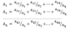
Where, a_ij∈[0,1] (1 ≤ i ≤ q, 1 ≤ j ≤ q), uj is the jth interval of the UoD. The value of a_ij denotes the degree of membership of uj in the fuzzy set A_i which are defined by the triangular membership function with three values 0, 0.5 and 1.
Step 5: Fuzzy the historical time series data into fuzzy sets A_i
Fuzzy time series is generated by converting each historical data into a fuzzy set. If a time series datum depends on interval u_j and the maximal membership value of fuzzy set A_i occurs at u_j, then the historical datum is considered as fuzzy set A_i. In this way, all historical data of time series is fuzzified into A_i.
Step 6: Define all β – order fuzzy logical relations (β ≥ 1 ).
The fuzzy logical relationship can be construct by two or several consecutive fuzzified values, respectively. To create an β- order FLR, we need to explore any relationship – type as F(t-β),F(t-β+1),…,F(t-1)→F(t), in which F(t-β),F(t-β+1),…,F(t-1) and F(t) are called the “current state” and the “next state” of the fuzzy logical relationship, respectively. Then, it has been obtained by replacing the corresponding fuzzy sets A_i.
Step 7: Establish all β – order fuzzy relationship groups (FRGs)
We use fuzzy relationship group [17] to form FRGs in this study. To clarify this, we consider three first – order FLRs at three different times t-2, t-1 and t as follows: 〖 A〗_i → 〖 A〗_j; 〖 A〗_i → 〖 A〗_k and 〖 A〗_i → 〖 A〗_j , respectively. Suppose that we want to forecast the value of time series data of time t-1, the appearance of the fuzzy sets on the right-hand side of FLRs having the same left – hand side is considered to form into together G1 as 〖 A〗_i→〖 A〗_j, 〖 A〗_k. The same way, if forecasting time t, the FLRs which have the same right-hand side are grouped into a group G2 as 〖 A〗_i→〖 A〗_j, 〖 A〗_k, 〖 A〗_j.
Step 8: Calculate and defuzzify the forecasted output values
To defuzzify the fuzzified time series data which are based on the established FRGs, we apply two rules which are introduced in papers [31, 14] to calculate the forecasting output values at time t as follows:
Rule 1: Applying for computing output values in the training stage
Our defuzzified principle in article [31] is employed to calculate value based on information of each group. For each group in the training stage, we divide each corresponding interval with regards to the fuzzy sets in the next state of the TV- FRGs into three sub-intervals with equal- length as calculated in (4)

where, n denotes the total number of fuzzy sets on the left-hand side of TV-FRG.
〖subm〗_ik denotes the medium value of one of three sub-intervals ( 1≤k≤3) with regards to i-th fuzzy set in the next state of FRG that the real data at forecasting time falls into this sub-interval.
〖Value_lu〗_ik denotes the one of two values belongs to lower or upper bound of one of three sub-intervals which has the real data at forecasting time ranges from L_ik to U_ik of sub-interval. If the real data value at forecasting time minor the mid-point value of sub-interval u_ik, then 〖Value_lu〗_ik is allocated as the lower bound of sub-interval u_ik; else 〖Value_lu〗_ik is allocated as the upper bound of sub-interval u_ik
Rule 2: Applying for calculating output value in the testing stage
In the testing stage, prediction value of each group which has the unknown linguistic value on the next state is estimated by the master vote scheme [14]. Assume there a β – order FRG which has type as A_(t-β) ,A_(t-(β+1)),A_t1→#, the prediction value is estimated according to (5) as follows:

Where , the symbol w_h is the highest votes predefined by user; is the order of the FLRs; the symbols M_(t-1), M_(t-2)… and M_(t-β) are the medium values corresponding to intervals in accordance to the latest fuzzy set and other fuzzy sets on the current state of FRG having the maximal membership values of A_(t-1), A_(t-2), …, and A_(t-β) occur at intervals u_t1, u_t2,…, and u_(t-β), respectively.
Step 9: Evaluate the performance of the proposed model
The forecasting performance of the proposed model estimated by two following criterions as: Mean Square Error (MSE) and Mean Absolute Percentage Error (RMSE).

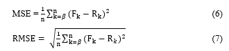
Here, R_k and F_k are the actual and forecasted value at time k, respectively, n is number of observations to be forecasted, β is the order of fuzzy relationship.
In the following, we propose a new approach for optimizing parameters of Hedge Algebras, called “Optimizing parameters of HA based on PSO”. This approach is utilized in Step 2 of the proposed model to get the optimal parameters of HA. Details of this approach are shown in Algorithm 2.
Algorithm 2: Optimizing parameters of HA based on PSO algorithm
Step 1: Initialize; Generate P particles in two – dimensional space
Assume that the fuzziness interval of “Low” term denotes the first dimension and fuzziness intervals of “Little” hedge denotes the second dimension in the construct HA.
Let kd be a particle including two elements l_(kd,1) and l_(kd,2), represented by the position vector L_kd=[l_(kd,1),l_(kd,2)]; where l_(kd,i)  [0, 1], 0 ≤ i ≤ 1 and l_(kd,1)+ l_(kd,2) = 1. These two elements act as the fuzziness intervals of fm(Low) and µ(Little) of HA, as given in Figure 2(a). The velocity of each particle kd is denoted by the velocity vector V_kd=[v_(kd,1),v_(kd,2)] including two elements v_(kd,1) and v_(kd,2) as shown in Figure 2(b).
In th PSO, the initial position vector L_kd and the initial velocity V_kd of each particle kd are generated randomly in range [0, 1], the personal best position vector P_(best,kd) =[p_(kd,1),p_(kd,2)] of each particle kd denoting the best position which has the minimum objective value found so far. Initially, the personal best position vector P_(best,kd) of each particle kd like its initial position vector L_kd.
l_(kd,1) l_(kd,2)

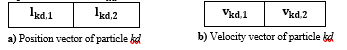Figure 2: The graphical representation of particle kd

Step 2: while (t ≤ iter) do // iter is a predefined number of iterations
For each particle kd do the following steps:
Step 2.1: Calculate the objective value 〖MSE〗_kd of each particle kd, as given by following sub-steps:
Step 2.1.1: Generate q linguistic terms corresponding to q intervals
From the position vector L_kd=[l_(kd,1),l_(kd,2)] or two parameters fm(Low) and µ(Little) of HA, divide the U into q intervals as u_1=[d_min- n_1,p_1], u_2=[p_1,p_2],…, u_k=[p_(q-1),d_max+ n_2], respectively.
Step 2.1.2: Based on the obtained intervals, define q fuzzy sets as A_1, A_2,…, A_(q-1) and A_q
Step 2.1.3: Fuzzy the historical time series data into fuzzy sets A_i
Step 2.1.4: Establish fuzzy relationships based on the fuzzy sets A_i defined and fuzzified data
Step 2.1.5: Establish all TV-FRGs based on FLRs defined
Step 2.1.6: Defuzzify and calculate the forecasting output values
Step 2.1.7: Compute the objective value 〖MSE〗_kd of each particle based on formula (6)
Step 2.2: Update the private best position vector P_(best,kd) of each particle kd, if MSE^t (kd) <= MSE^(t-1) (kd); p_(kd,1) 〖=l〗_(kd,1)and p_(kd,2) 〖=l〗_(kd,2)
Step 2.3: Choose the best particle Gbest among all P particles, (which has the minimum MSE value), set P_Gbest = [l_(Gbest,1), l_(Gbest,2)] be the position vector of the Gbest
Step 2.4: Update the velocity V_kd and the position L_kd of each particle kd according to (1) and (2), respectively; update ? in (3).
end for
Step 3: Check the stopping criterion
If (t < iter), then let t = t+1 and go to Step 2.1 else, print the results ( the position vector P_Gbest = [l_(Gbest,1), l_(Gbest,2)] be the optimal parameters of HA by letting Fm(Low) = l_(Gbest,1) and µ(Little) = l_(Gbest,2))).
end while
To sum up, the flowchart of the proposed algorithm “Optimizing parameters of HA based on PSO”, which is shown in Figure 3.
Next, we present algorithm “Finding optimal intervals using PSO” which has been called in Step 3 of the proposed model to find the best length of each interval with view to getting the better accurate forecasting.
Finding optimal intervals using PSO
In this algorithm, PSO is used to adjust the initial interval lengths which are determined by Algorithm 2. The briefly explanations of this algorithm are given as below: Each particle of PSO in q-dimensional space is used to represent the partitioning of time series data, where q is the number of intervals in the UoD. Assume that the lower bound and upper bound of UoD be p_0= (d_min- n_1) and p_q =(d_max+ n_2), respectively. Each particle represents a vector including q-1 elements as p_(kd,1), p_(kd,2), …, p_(kd,q-2) and p_(kd,q-1), where (1≤i≤ q-1) and p_(kd,i)≤ p_(kd,i+1). From q-1 elements, attain the q adjoining intervals as u_1=[p_0,p_(kd,1)], u_2=[p_(kd,1),p_(kd,2)],…,u_q=[p_(kd,q-1),p_(kd,q) ], respectively. If particles in a swarm move to from current position to another, the elements of the new vector with regards to position of particles that need to be adjusted in an ascending order (p_(kd,1)≤ p_(kd,2)≤⋯≤ p_(kd,q-1)). In the training phase, position of each particle is changed by using (1) and (2), and repeated the steps until the repeated value (t) equal to the predefined number of iterations (iter). If (t = iter), then all the FRGs obtained by the (Gbest) among all personal best positions (P_(best_kd)) of all particles which used to forecast the new data in testing phase and presented in Algorithm 4. Here, the MSE function in (6) is used to represent the forecasting accuracy of each particle in the training stage. The steps of the algorithm “Finding optimal intervals using PSO” are shown in Algorithm 3 as follows:
Algorithm 3: Finding optimal intervals using PSO
Input: Historical time series data
Output: Optimal intervals and the MSE value
Initialize:
P particles in q-dimensional space, the maximum iteration (iter)
The initial position Pkd and the velocity Vkd of all particles, respectively. Where, the intervals in position vector is created by the particle 1 be the same as the one which are created from HA as u_1=[p_0,p_1,1], u_2=[p_1,1,p_1,2],…,and u_q=[p_(1,q-1),p_(1,q)],
The initial personal best position vectors of the kdth particle is the same as its initial position vector at the beginning: let P_(best,kd) = P_kd
while (t ≤ iter) do // iter is maximum iteration number
for each particle kd (1≤kd≤P) do
Calculate the objective value 〖MSE〗_kd, of each particle kd by performing the steps from Step 4 to Step 8 above, such as: defining fuzzy sets, fuzzify time series data, determining all β- order fuzzy relations, establishing all β- order TV- FRGs, computing forecasted values
Update P_(best,kd) value of particle kd by the MSE values
P_(best,kd)^(t+1) ={█(P_(best,kd)^(t+1) ; &if MSE(P_kd^(t+1) )>P_(best,kd)^t@MSE(P_kd^(t+1) ) ; & if MSE(P_kd^(t+1) ) ≤P_(best,kd)^t )┤
End for
Update the global best position G_best by the MSE value.
for each particle kd (1≤kd≤P) do
Update the velocity: V_(kd,i)^(t+1)= ω^t* V_(kd,i)^t+c_1*R1( )*(P_(best,kd)-P_(kd,i)^t )+c_2*R2( )*( G_best-P_(kd.i)^t )
Update the position: P_(kd.i)^(t+1)=P_(kd,i)^t+V_(kd,i)^(t+1)
End for
Update inertia weight ω : ω^(t )=ω_(max )-(t*( ω_max-ω_min))/iter
End while
Instance: Explanation of the optimization process of the proposed model using Algorithm 3 on the enrolments data [4] is given as follows: the number of intervals and particles corresponding be (q = 7 and P=4, respectively. From the historical enrolments data, we define the UoD as U = [13000, 20000], where lower bound p_0 = 13000 and upper bound p_7= 20000, respectively. For finding the optimal solution, the parameters in PSO is defined as: the values of p_(kd,i) fall within the range of (13000, 20000], the values of v_(kd,i) fall within the range of [-100, 100], (1≤ i ≤ 7, 1≤ kd ≤ 4), the values of C_1 and C_2 be 2, and the ? value ranges from 0.9 to 0.4 and maximum number of iterations be 2, respectively. The positions and velocities of all particles are initialized randomly and listed in Tables 1 and 2, respectively.
Algorithm 4: The forecasting algorithm in the testing stage
The optimal lengths of intervals and order of FLRs obtained in Algorithm 3 that are used to estimate untrained data in the testing stage based on the Principle 2 in the forecasting model.
In Table 1, we have given the 7 intervals for 4 particles which are u_1=[p_0,p_1], u_2=[p_1,p_2],…, and u_7=[p_6,p_7], respectively. Where, the initial position of particle 1 act as the intervals are created as the same the one which are obtained from HA in Algorithm 2 and listed as u_1= [13000, 14470.47), u_2= [14470.47, 15149.8) , u_3= [15149.8, 15829.15), u_4= [15829.15, 16143), u_5= [16143, 16528.14), u_6= [16528.14, 17361.8), u_7= [17361.8, 20000]. The MSE value of particles is considered according to equation (6). From the corresponding MSE values, every particle records its own personal best positions (P_best) so far.

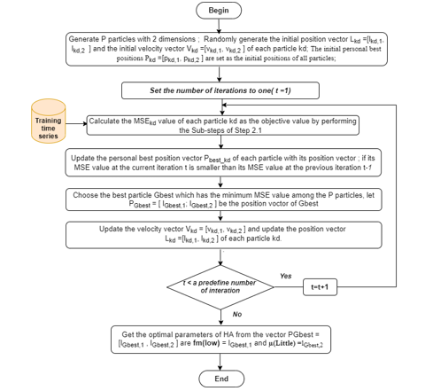Figure 3: Flow chart of the proposed algorithm “Optimizing parameters of HA based on PSO”

Table 1: The randomized initial positions of all particles

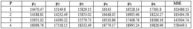
Table 2: Randomly generated initial velocities of all particles

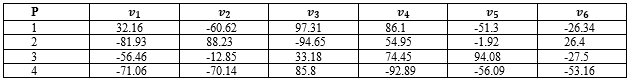
Table 3: The initial Pbest of all particles; the Gbest value is created by particle 1.

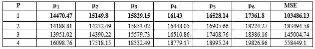
Table 4: The second positions of all particles

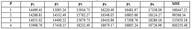
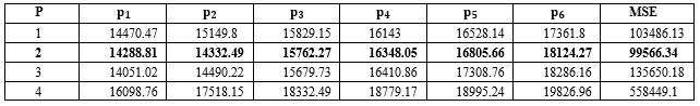
Table 5: The second Pbest of all particles; the Gbest value is obtained by particle 2

Firstly, the P_best values are initialized to the same as the initial position of all particles. Table 3 presents the P_best values of all particles so far and the global best position Gbest = min (P_best) which is particle 1. After the first iteration, all particles change its positions based on (1) and (2). The second positions and the corresponding new MSE values of all particles are presented in Table 4.
Comparing the MSE values in Table 3 with the MSE values in Table 4, it can be seen that particle 2 and particle 3 in Table 4 attained a better position than their own P_best values so far. Thus, the two particles are updated in Table 5. The new Gbest is obtained by particle 2, because of the its smallest MSE value. The proposed model is accomplished by repeating the steps in Algorithm 3 until the maximal number of iterations is reached. Finally, the proper lengths of intervals are achieved corresponding to Gbest value that the particle 2 gets so far. These obtained intervals are employed to forecast the final output results.

Experiments and analysis

In this paper, our forecasting model has been implemented on two datasets as enrolments data of University of Alabama [3] and number of deaths in car road accidents in Belgium [32]. These two datasets have been applied for forecasting with the huge amount of research works in the literature. Before implementing the proposed forecasting model, two time series datasets are briefly described. Then, the simulated results and analyses related to these datasets are given, respectively. Description of time series data and evaluation of the proposed model are discussed as follows.
Prepare data for experiments
Time series description
This study, we focus on two time series datasets which are often used to demonstrate validity and performance of the FTS forecasting model. The statistical characteristics of two these time series are expressed as follows.
The enrolments dataset of university of Alabama
This time series data consists of 22 values between 1971 and 1992, see Figure 4(a). This dataset has utilized to examined with the huge amount of reseach works which are presented in the articles [1, 2, 4, 6 – 7, 10 -12, 14, 15, 17, 21 – 24, 29 – 31]. The obtained results among these works are choosed for comparing with our proposed model. Some of results among these studies are considered for comparing with that of the proposed model in this paper. The UoD of enrolments time series is determined as U=[d_min- n_1,d_max+ n_2] = [13000, 20000].
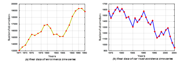Figure 4: Plots of the amplitude of time series used in experiments

In which, the minimal value and the maximal are d_min=13055 and d_max=19337, respectively, and two proper positive values n_1 and n_2 are set as 55 and 663, respectively
The dataset of car road accidents in Belgium
There are 31 observations about the car road accidents ranges from 1974 to 2004 that taken from National Institute of Statistics, Belgium. Figure 4(b) depicts the yearly deaths in car road accidents in Belgium. This time series data is investigated in the research works [6, 32, 40 – 42]. The obtained results from these works have been also selected to compare with our proposed model. In this time series, the minimal value and the maximal are d_min= 953 and d_max=1644, and two proper positive values n_1 and n_2 are set as 3 and 6, respectively. Therefore, the UoD can be defined as U=[d_min- n_1,d_max+ n_2] = [950, 1650].
Table 6: The parameters of PSO are applied to the enrolments data and car road accidents data

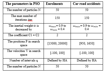
Setup parameters for experiments
For implementing the experiments, we use C# programming tool on an Intel Core i7 PC with 8GB RAM. From parameters of each time series data in Table 6, our forecasting model is tested 30 independent runs on each of dataset with various number of orders and intervals to make forecasting results. Then, the best result of among testing runs is recorded to compare with most well-known models in the same dataset with regards to MSE (6) and RMSE (7) functions. The selected parameters of the PSO are used in experiments for receiving optimal intervals and final forecasting results are placed in Table 6.
Application of forecasting and comparing results
In this section, we give out results of two experiments with regards to real-world time series datasets which are described in Section 4.1. Then, comparison of results between the proposed model and well-known FTS models in the literature are also presented.
Applying for Experiment 1
Case (1): Forecasted results obtained by the first – order FTS
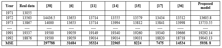
The forecasting results obtained from this experiment are compared with the ones of the current models [34-37, 27, 29] under the same number of intervals equal to 7. A comparison with regards to RMSE value between the proposed model and the different forecasting models are given in Table 7. Considering the Table 7, the results show that the proposed model has the smallest forecasting errors with regards to RMSE value equal to 188.8 among all its counterparts. There are significant differences between the proposed model and the compared models above. It is the way which determining of the fuzzy relationship group and method of partitioning the UoD are applied in the forecasting model. Three models in works [34-36] are constructed according to the framework [3] to forecast different problems and apply information granules for partitioning, respectively, whereas the proposed model uses hedge algebras for determining unequal-sized interval lengths. Comparing with two models in articles [27, 29]. These models apply the fuzzy relation groups [3] to structure the forecasting model, in which the proposed model uses the fuzzy relation groups that we have proposed in article [17] to build the forecasting model. Comparing the model [37], the proposed model employs the HA combining with PSO to select the optimal intervals, whereas the model [37] applies the maximum spanning tree based fuzzy clustering for dividing intervals with different lengths in the intuitionistic FTS model. In addition, the proposed model is also given to compare with other models which are presented in [6, 11, 14, 15, 17, 36, 38] under the number of intervals of 14. The forecasting results and MSE values between our model and other models are given in Table 8. Table 8 shows that our model has capable of more accurate forecasting and obtains the MSE value 5938.8 which is the smallest among all the existing models.

Table 7: Comparative results of proposed model with the current models based on first – order FTS under seven intervals

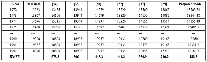
Table 8: Comparative results of the proposed model with the current models based on first – order FTS with number of intervals of 14

Case (2): Forecasting results obtained by the high – order FTS
In this case, all historical enrolments dataset [4] covering a period from year 1971 to 1992 are separated into two parts. The first part including 19 observations between 1971 and 1989 is used for training and the second part consists of 3 observations is utilized for testing. The forecasting performance of our model and the compared models are evaluated using the MSE and RMSE function.
The obtained results in the training stage
To authenticate the superiority of our prediction model based on the different high – order FLRs, the research works [7, 12, 14, 15, 17] are cited for comparing. The comparative results for all forecasting models under the number of intervals equal to 7 are shown in Table 9. From Table 9 shows that the proposed model outperforms in term of forecasting accuracy the other existing models under different high-order fuzzy relationships at all. In particularly, our model has the smallest average MSE value of 1608.26 among all of compared models. Among all fuzzy relationships is done in the model, the proposed model obtains the lowest MSE value equal to 111.6 by 6th- order fuzzy relationships. The major difference between our model and the compared models is approach of forming FRGs and optimization method they used. In optimization method, the model [12] performs genetic algorithm but the models in articles [14, 15, 17] and the proposed model proceed the PSO algorithm to achieve the best intervals, respectively. Also using PSO to find suitable intervals, our model incorporates HA to partition the different initial intervals of the UoD instead of equal length intervals. In the determining of FRGs, our model is constructed from model [17], the remaining models in articles [7, 12, 14, 15] are created from structure [3]. From the above analysis, it is clearly seen that our model provides more convincing forecasted results when compared to five models considered above.
In addition, our proposed model has been also applied to compare with other existing models based on the different high–order FTS under number of intervals equal to 14. These compared models which are presented in papers [7, 39,12, 14, 15]. The comparative results of the proposed model with its counterparts are placed in Table 10. Comparing model [39] with the proposed model, the proposed model provides the better MSE value. In addition, comparing the forecasting model in article [7] and the proposed model, both of them use the 5th-order fuzzy relationship but our model is much more superior in term of forecasting accuracy. When compared with remaining forecasting models in articles [12, 14, 15]. Although these modes use the fuzzy logical relationship with number of orders is larger, but the results obtained from our model are also better than the existing competing models. In particular, from Table 10, our model obtains the forecasting error MSE of 16.9 which is the lowest among five compared models above. This can conclude that the proposed model not only provides superior forecasting results but also shows the best stability based on the various high-order FLRs, for all cases. To be clearly imagined, Figure 5 describes the trend in term of forecasting accuracy between our model and the previous models for different orders. Viewing these curves, it is clearly seen that forecasting accuracy of our model is more accurate than those of compared models under dissimilar high-order FLRs at all. To sum up, the comparisons above is enough to demonstrate the effectiveness of our model which outpace the previous models based on high – order model with unlike number of intervals in the forecasting the enrolments of University of Alabama.

Table 9: The results of the our model and the compared models with 7 intervals

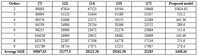
Table 10: The obtained results of our model and the compared models with 14 intervals

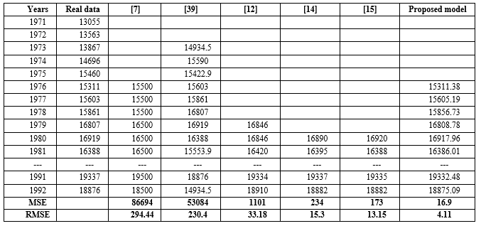
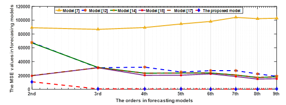Figure 5: The curves of the MSE values between the our model and the compared models

The obtained results in the testing stage
From enrolments time series from 1971 to 1992, to forecast the new enrolments for the next year with one head – step. Can be explained through the examples as below: the historical data of enrolments from year 1971 to 1989, is utilized to forecast the new enrolment of year 1990. In the same way, the enrolments data between 1971 and 1990 are used to forecast data of year 1991. Thereafter the enrolments data have been well trained by our model, the future enrolments values could be accomplished to compare to the future ones of the forecasting models proposed in articles [4, 11, 14, 39]. A comparative forecasting results produced by the 3rd – order FTS with different number of intervals and the highest vote 〖 W〗_h=15 [14] which are shown in Table 11 and 12. From these Tables show that our model obtains the smallest RMSEs value equal to 99.2 and 60.28 among five competing models, respectively.
Table 11: Comparative results of our model with other models under the number of intervals of 7 and which use vote〖 W〗_h=15

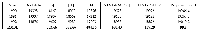
Table 12: Comparative results of our model with other models under the number of intervals of 14 and which use vote〖 W〗_h=15

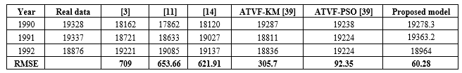
Table 13: The obtained results between our model and the competing models using the different number of intervals and various orders

Applying for Experiment 2

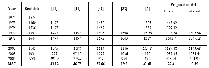
In this section, our proposed model have been implemented for forecasting the car road accidents in Belgium [32] ranges period from 1974 to 2004. We also test 30 times and take the best forecasting result to compare with the results from the other five forecasting models in articles [40 – 42, 32, 6]. The comparative results based on the different number of intervals and the various orders of FTS are shown in Table 13. Comparing between models [40, 6] and our proposed model, our model achieves the far better MSE value of 29.4 in two compared models based on the first – order FTS with different number of intervals. Also, from Table 13, we can be seen that, comparing model [41] and model [32], our proposed model produces the far smaller MSE value of 0.85 in two considered competing models using the 3rd – order FTS with different number of intervals. To summarize, the our model provides better forecasting results and higher accuracy than the models in [40 – 42, 32, 6] corresponding to the number of orders of FTS and number of intervals equal to 14 as shown in Table 13.

Conclusions and upcoming work

In this paper, a novel model for predicting enrolments and car road accident is developed. To remedy the downside of the conventional FTS model, the FTS proposed model combines hedge algebras and PSO is developed to resolve two issues which are considered to be important and greatly affect the forecasting accuracy is that the length of intervals and fuzzy relationship group. By utilizing the concept of time variant fuzzy relationship group, the proposed model has handled the more persuasive historical data and has been demonstrated to be more appropriate for real-world applications. In addition to that the parameters of HA are modified by PSO algorithm to get the initial intervals partitioning of the UoD. In data mining and finding of optimal solution, PSO is considered to accomplish better compared to other heuristic techniques with regards to success rate and solution quality. Furthermore, the forecasting efficiency of the proposed model is significantly improved in adjusting the lengths of intervals. The forecasting performance of the proposed model is demonstrated by forecasting the enrolments at University of Alabama and the car road accidents in Belgium. Details of the comparison in Tables 7-13 indicate that the proposed model achieves the lowest forecasting errors when compared with other forecasting models., for many cases. Also, from Figure 5, it can be observed that the amount of error rate in terms of MSE obtained by our high – order FTS model are smaller than all other models considered in this research. Even though our model shows that the greater forecasting capability when compared with some of recent ones based on the high-order FLRs. Determining of the high-order FLR spends a lot of computational time than first-order FLR. Therefore, development of new approaches that can automatically select out the optimal degree of the high-order FLRs is a worthy idea in FTS forecasting model. Those will be the work closely related to this research in the coming time.

Acknowledgment

This study was supported in the Science Council of Thai Nguyen University of technology (TNUT), Thai Nguyen, Vietnam.

1. Q. Song, B.S. Chissom, “Fuzzy time series and its models”, Fuzzy Sets and Systems, 54(3), 269-277, 1993a, http://dx.doi.org/10.1016/0165-0114(93)90372-O.
2. Q. Song, B.S. Chissom, “Forecasting Enrollments with Fuzzy Time Series – Part I,” Fuzzy set and systems, 54(1), 1-9, 1993b, http://dx.doi.org/10.1016/0165-0114(93)90355-L.
3. L.A. Zadeh, “Fuzzy sets”, Information systems, 8, 338–353, 1965, http://dx.doi.org/10.1016/S0019-9958(65)90241-X.
4. S.M. Chen, “Forecasting Enrollments based on Fuzzy Time Series,” Fuzzy set and systems, 81, 311-319, 1996, http://dx.doi.org/10.1016/0165-0114(95)00220-0.
5. H.K. Yu “Weighted fuzzy time series models for TAIEX forecasting ”, Physica A, 349 , 609–624, 2005.
6. V.R. Uslu, E. Bas, U.Yolcu, E. Egrioglu, “A fuzzy time series approach based on weights determined by the number of recurrences of fuzzy relations”, Swarm and Evolutionary Computation, 15, 19-26, http://dx.doi.org/10.1016/j.swevo.2013.10.004, 2014.
7. S. M. Chen, “Forecasting Enrollments based on hight-order Fuzzy Time Series”, Int. Journal: Cybernetic and Systems, 33(1), 1-16, 2002, http://dx.doi.org/10.1080/019697202753306479.
8. K. Huarng, “Effective lengths of intervals to improve forecasting in fuzzy time series”. Fuzzy Sets and Systems, 123 (3) , 387–394, 2001b, http://dx.doi.org/10.1016/S0165-0114(00)00057-9
9. L. W. Lee, L. H. Wang, S. M. Chen, Y.H. Leu, “Handling forecasting problems based on two-factors high-order fuzzy time series”. IEEE Transactions on Fuzzy Systems, 14, 468–477, 2006.
10. S.M. Chen, K Tanuwijaya “Fuzzy forecasting based on high- order fuzzy logical relationships and automatic clustering techniques”, Expert Systems with Applications, 38, 15425–15437, 2011.
11. S.M. Chen, N.-Y. Chung, “Forecasting enrollments of students by using fuzzy time series and genetic algorithms”, International Journal of Information and Management Sciences, 17, 1–17, 2006a.
12. S.M. Chen, N.-Y. Chung, “Forecasting enrollments using high-order fuzzy time series and genetic algorithms”, International of Intelligent Systems, 21, 485–501, 2006b.
13. L.-W. Lee, L.-H. Wang, S.M. Chen, “Temperature prediction and TAIFEX forecasting based on high order fuzzy logical relationship and genetic simulated annealing techniques,” Expert Systems with Applications, 34, 328–336, 2008.
14. I. H. Kuo, S. J. Horng, T.W. Kao, T.L, C.L. Lee, Y. Pan, “An improved method for forecasting enrollments based on fuzzy time series and particle swarm optimization”, Expert systems with applications, 36, 6108–6117, 2009, http://dx.doi.org/10.1016/j.eswa.2008.07.043.
15. Y.L. Huang, S. J. Horng, M. He, P. Fan, T.W. Kao, M.K. Khan, J.L. Lai, I. H.Kuo, “A hybrid forecasting model for enrollments based on aggregated fuzzy time series and particle swarm optimization”. Expert Systems with Applications, 38, 8014–8023, 2011.
16. L.Y. Hsu, S.J. Horng, T.W. Kao, Y.H. Chen, R.S. Run, R.J. Chen, J.L. Lai, I. H.Kuo, “Temperature prediction and TAIFEX forecasting based on fuzzy relationships and MTPSO techniques”, Expert Syst. Appl., 37, 2756–2770, 2010.
17. N.C. Dieu, N.V. Tinh, “Fuzzy time series forecasting based on time-depending fuzzy relationship groups and particle swarm optimization”, In: Proceedings of the 9th National conference on Fundamental and Applied Information Technology Research (FAIR’9), Can Tho, Vietnam, 125-133, 2016, doi: 10.15625/vap. 2016.00016.
18. J.I.Park, D.J. Lee, C.K.Song., M.G. Chun, “TAIFEX and KOSPI 200 forecasting based on two-factors high-order fuzzy time series and particle swarm optimization”, Expert Systems with Applications, 37, 959–967, 2010
19. S.M. Chen, H.P. Bui Dang, “Fuzzy time series forecasting based on optimal partitions of intervals and optimal weighting vectors”, Knowledge-Based Systems, 118, 204–216, 2017.
20. S.M. Chen, W.S. Jian, “Fuzzy forecasting based on two-factors second-order fuzzy-trend logical relationship groups, similarity measures and PSO techniques”, Information Sciences, 391–392, 65–79, 2017.
21. M. Bose, K. Mali, “A novel data partitioning and rule selection technique for modelling high-order fuzzy time series”, Applied Soft Computing, 17, 1-15, https://doi.org/10.1016/j.asoc.2017.11.011, 2017.
22. Z.H.Tian, P.Wang, T.Y. He, “Fuzzy time series based on K-means and particle swarm optimization algorithm”, Man-Machine-Environment System Engineering. Lecture Note in Electrical Engineering. 406, 181-189, Springer 2016.
23. Z. Zhang, Q. Zhu. “Fuzzy time series forecasting based on k-means clustering”, Open Journal of Applied Sciences, 2, 100-103, 2012.
24. N.V. Tinh, N.C. Dieu, “Improving the forecasted accuracy of model based on fuzzy time series and k-means clustering”, journal of science and technology: issue on information and communications technology, 3(2), 51-60, 2017.
25. E.Bulut, O. Duru, S.Yoshida, “A fuzzy time series forecasting model formulti-variate forecasting analysis with fuzzy c-means clustering”, WorldAcademy of Science, Engineering and Technology, 63, 765–771, 2012.
26. S. Askari, N. Montazerin, “A high-order multi-variable Fuzzy Time Series forecasting algorithm based on fuzzy clustering”, Expert Systems with Applications, 42, 2121–2135, 2015.
27. N.C. Ho, N.C. Dieu, V.N. Lan. “The application of hedge algebras in fuzzy time series forecasting”, Journal of science and technology, 54(2), 161-177, 2016.
28. N.C. Ho., W. Wechler,“Hedge algebra: An algebraic approach to structures of sets of linguistic truth values”, fuzzy Sets and Systems, 35, 281-293, 1990.
29. H.Tung, N.D. Thuan, V.M. Loc, “The partitioning method based on hedge algebras for fuzzy time series forecasting”, Journal of Science and Technology, 54 (5), 571-583, 2016.
30. N.D. Hieu , N.C. Ho, V.N. Lan, “Enrollment forecasting based on linguistic time series”, Journal of Computer Science and Cybernetics, 36(2), 119-137, 2020.
31. N.V. Tinh, “Enhanced Forecasting Accuracy of Fuzzy Time Series Model Based on Combined Fuzzy C-Mean Clustering with Particle Swam Optimization”, International Journal of Computational Intelligence and Applications, 19(2), 1-26, 2020.
32. S M. Yusuf, M.B. Mu’azu, O. Akinsanmi, “ A Novel Hybrid fuzzy time series Approach with Applications to Enrollments and Car Road Accident”, International Journal of Computer Applications, 129(2):37 – 44, 2015.
33. J. Kennedy, R. Eberhart, “Particle swarm optimization”, Proceedings of IEEE international Conference on Neural Network, 1942–1948, 1995.
34. L.Wang, X. Liu, W. Pedrycz. “Effective intervals determined by information granules to improve forecasting in fuzzy time series”. Expert Systems withApplications, 40, pp.5673–5679, 2013.
35. L. Wang, X. Liu, W. Pedrycz, Y. Shao, “Determination of temporal information granules to improve forecasting in fuzzy time series”. Expert Systems with Applications, 41(6), 3134–3142, 2014, http://dx.doi.org/10.1016/j.eswa.2013.10.046.
36. W. Lu, X. Chen, W. Pedrycz, X. Liu, J. Yang, “Using interval information granules to improve forecasting in fuzzy time series”. International Journal of Approximate Reasoning, 57, 1–18, 2015.
37. Y. Wang, Y. Lei, X. Fan, Y. Wang, “Intuitionistic Fuzzy Time Series Forecasting Model Based on Intuitionistic Fuzzy Reasoning”, 2016, Article ID 5035160 , pp 1-12, 2016, DOI: 10.1155/2016/5035160.
38. Abhishekh, S. S. Gautam, S. R. Singh, “A refined weighted method for forecasting based on type 2 fuzzy time series”, International Journal of Modelling and Simulation, 38(3), 180-188, 2018, doi.org/10.1080/02286203.2017.1408948.
39. K. Khiabani, S.R. Aghabozorgi, “Adaptive Time-Variant Model Optimization for Fuzzy-Time-Series Forecasting”, IAENG International Journal of Computer Science, 42(2), 1-10, 2015.
40. T A. Jilani, S. M .Burney., C. Ardil, “Multivariate high order FTS forecasting for car road accident”, World Acad Sci Eng Technol, 25, 288 – 293, 2008.
41. Jilani T A, Burney S M A. Multivariate stochastic fuzzy forecasting models”. Expert Syst Appl, 353, 691–700, 2008
42. E.Bas, V. Uslu. , U.Yolcu, E. Egrioglu, “A modified genetic algorithm for forecasting fuzzy time series”, Appl Intell, 41, 453-463, 2014.

Citations by Dimensions

Citations by PlumX

Google Scholar

Crossref Citations

1. Almahasees Zakaryia, Al-Taher Mohammad, Helene Jaccomard, "Evaluation of Facebook Translation Service (FTS) in Translating Facebook Posts from English into Arabic in Terms of TAUS Adequacy and Fluency during Covid-19", Advances in Science, Technology and Engineering Systems Journal, vol. 6, no. 1, pp. 1241–1248, 2021. doi: 10.25046/aj0601141
2. Eko Subiyantoro, Ahmad Ashari, Suprapto, "Learning Path Recommendation using Hybrid Particle Swarm Optimization", Advances in Science, Technology and Engineering Systems Journal, vol. 6, no. 1, pp. 570–576, 2021. doi: 10.25046/aj060161
3. Abdurazaq Elbaz, Muhammet Tahir Güneşer, "Optimal Sizing of a Renewable Energy Hybrid System in Libya Using Integrated Crow and Particle Swarm Algorithms", Advances in Science, Technology and Engineering Systems Journal, vol. 6, no. 1, pp. 264–268, 2021. doi: 10.25046/aj060130
4. El hadji Mbaye Ndiaye, Mactar Faye, Alphousseyni Ndiaye, "Comparative Study Between Three Methods for Optimizing the Power Produced from Photovoltaic Generator", Advances in Science, Technology and Engineering Systems Journal, vol. 5, no. 6, pp. 1458–1465, 2020. doi: 10.25046/aj0506175
5. Mohamed Hedi Fourati, Soumaya Marzouk, Mohamed Jmaiel, Tom Guerout, "Docker-C2A : Cost-Aware Autoscaler of Docker Containers for Microservices-based Applications", Advances in Science, Technology and Engineering Systems Journal, vol. 5, no. 6, pp. 972–980, 2020. doi: 10.25046/aj0506116
6. Trinh Luong Mien, Vo Van An, Bui Thanh Tam, "A Fuzzy-PID Controller Combined with PSO Algorithm for the Resistance Furnace", Advances in Science, Technology and Engineering Systems Journal, vol. 5, no. 3, pp. 568–575, 2020. doi: 10.25046/aj050371
7. Houcine Marouani, Amin Sallem, Mondher Chaoui, Pedro Pereira, Nouri Masmoudi, "Multiple-Optimization based-design of RF Integrated Inductors", Advances in Science, Technology and Engineering Systems Journal, vol. 4, no. 4, pp. 574–584, 2019. doi: 10.25046/aj040468
8. Selma Tchoketch Kebir, Mohamed Salah Ait Cheikh, Mourad Haddadi, "A detailed step-by-step electrical parameters identification method for photovoltaic generators using a combination of two approaches", Advances in Science, Technology and Engineering Systems Journal, vol. 3, no. 4, pp. 45–52, 2018. doi: 10.25046/aj030406
9. Sahbi Marrouchi, Nesrine Amor, Moez Ben Hessine, Souad Chebbi, "Theoretical Investigation of Combined Use of PSO, Tabu Search and Lagrangian Relaxation methods to solve the Unit Commitment Problem", Advances in Science, Technology and Engineering Systems Journal, vol. 3, no. 1, pp. 357–365, 2018. doi: 10.25046/aj030144
10. Hossein Soleymani, Amin Hasanvand, "Estimation of Power System Stabilizer Parameters Using Swarm Intelligence Techniques to Improve Small Signal Stability of Power System", Advances in Science, Technology and Engineering Systems Journal, vol. 2, no. 4, pp. 139–144, 2017. doi: 10.25046/aj020419
11. Kamel Smiri, Habib Smei, Nourhen Fourati, Abderrazak Jemai, "Fault-Tolerant in Embedded Systems (MPSoC): Performance Estimation and Dynamic Migration Task", Advances in Science, Technology and Engineering Systems Journal, vol. 2, no. 3, pp. 1188–1195, 2017. doi: 10.25046/aj0203150
12. Pedro Acevedo, Martín Fuentes, Joel Durán, Mónica Vázquez, Carlos Díaz, "Pulse Generator for Ultrasonic Piezoelectric Transducer Arrays Based on a Programmable System-on-Chip (PSoC)", Advances in Science, Technology and Engineering Systems Journal, vol. 2, no. 3, pp. 205–209, 2017. doi: 10.25046/aj020327