On Adversarial Robustness of Quantized Neural Networks Against Direct Attacks

Adv. Sci. Technol. Eng. Syst. J. 9(6), 30–46 (2024);
 DOI: 10.25046/aj090604
Deep Neural Networks (DNNs) prove to be susceptible to synthetically generated samples, so-called adversarial examples. Such adversarial examples aim at generating misclassifications by specifically optimizing input data for a matching perturbation. With the increasing use of deep learning on embedded devices and the resulting use of quantization techniques to compress deep neural networks, it is critical to investigate the adversarial vulnerability of quantized neural networks.In this paper, we perform an in-depth study of the adversarial robustness of quantized networks against direct attacks, where adversarial examples are both generated and applied on the same network. Our experiments show that quantization makes models resilient to the generation of adversarial examples, even for attacks that demonstrate a high success rate, indicating that it offers some degree of robustness against these attacks. Additionally, we open-source Adversarial Neural Network Toolkit (ANNT) to support the replication of our results.
1. Introduction
This paper builds upon our recent work, presented at the 5th ACM/IEEE International Conference On Automation of Software Test [1], which involved a comprehensive study on transferability of adversarial examples among quantized networks under various conditions. In this study, we advance the analysis by examining the efficiency of adversarial attacks on quantized networks when attacks are created and applied on the same network (direct attacks). Together, our previous and current work provide a more complete understanding of how quantization affects network vulnerability by addressing both transfer-based and direct attack scenarios.
Adversarial examples are images with deliberately added per- turbations which can cause a network to misclassify the image at a high rate [2]. These perturbation vectors are computed using specific algorithms and often distort an image in such a way that it looks benign or clean to human observers but are enough to cause a network to misclassify the image [3, 4].
As the use of DNNs proliferates over various safety-critical domains like medical diagnosis [5], railway [6], and aviation [7], the possibilities of adversarial examples coercing a network into making adversary-controlled decisions become a severe threat. One of the domains where deep learning is rapidly gaining popularity is the embedded systems. For instance, autonomous systems use AI
for decision-making by processing sensory information [8], mobile devices use them for image processing [9], and surveillance systems use them for biometric analysis [10]. However, the implementation of deep learning on edge devices is challenging. While the em- bedded devices are inherently constrained in terms of memory and power resources [11, 12], the state-of-the-art capabilities of DNNs come at a price of tremendous computational power required for running them. A pre-trained neural network comes with a large number of parameters: AlexNet [13] has 60 million parameters; VGG16 [14], an improvement over AlexNet, has 138 million pa- rameters; similarly, ResNet50 [15], another popular DNN, has 26 million parameters. The presence of these large number of pa- rameters mean that the computational demand at run-time is very high and requires the systems implementing these models to have considerable computing capabilities for a smooth operation.
One of the solutions to the limited resource problem is using a high-performance server that handles the deep learning tasks, with the devices just having to communicate with the server. Another solution, which is more widely adopted, is to deploy optimized ver- sions of a base model on the device itself. On-device deployments has several benefits [16]:
- No need to communicate with the server frequently which saves energy.
- Privacy is maintained as the user data does not leave the
- Performance is improved as round-trips to the server is
Various methods have been developed to optimize models for on- device deep learning [17, 18, 19]. One such effective approach is model compression through quantization [20], which reduces both the computational complexity and memory footprint of a network by lowering the precision of its values from the default 32-bit floating point (float32) to smaller bitwidths.
However, recent studies have shown that quantized networks remain vulnerable to adversarial examples [21, 22]. The adversar- ial vulnerability is especially concerning in compressed networks because of the wide-spread use and accessibility of embedded de- vices as compared to the full-scale networks running on high-end servers. Moreover, adversarial examples are found to be transfer- able [4, 23, 24, 25]. Samples created in one network (source) are found to be effective when applied on another network (target) trained to perform similar tasks. Our prior work [1] investigated this transferability property. Interestingly, we observed that iterative attacks like the Boundary Attack [26] and Carlini-Wagner (CW) attack [27] showed high efficiency in direct attack settings (where the source and target network are same), even when the networks were quantized. In this paper, we present an in-depth analysis of this behaviour, offering further insights into attack effectiveness on quantized networks.
Our contributions with this work are as follows:
- We consider diverse adversarial attack algorithms to assess the adversarial vulnerability of quantized networks against direct Our analysis shows that even though some attacks succeed with high rate, quantized networks, in general, offer some resistance against both gradient-based and gradient-free attacks as they require higher distortion to become effective, making samples easier to detect.
- We introduce the Adversarial Neural Network Toolkit (ANNT), a holistic application that streamlines the entire process—from training full-precision and quantized models to generating adversarial examples and evaluating robust- ness—within a single ANNT, together with the trained models and adversarial images provided with this paper, en- ables the replication of our results—both from this study and our previous work [1]. Furthermore, ANNT can serve as a valuable resource for the research community, simplifying ex- perimentation by allowing users to train quantized models and immediately test their robustness using various adversarial attacks without switching between tools.
2. Scope of the Study
Only untargeted misclassifications are considered. This means, for an attack algorithm, classification to any class other than the true class is considered as a successful attack. Targetted misclassifications that require attack algorithms to cause misclassifications to a specific target class selected by an adversary are not considered.
When quantizing a network, both activation and weight values are quantized to the same bitwidth. Quantization of activation and weights individually to different bitwidths is possible and could be a subject of further work. Moreover, gradients and bias values are not quantized.
Further, the study is limited to only image classifiers. Datasets, attack algorithms, and DNNs are selected accordingly.
3. Background
3.1. Deep Neural Network (DNN)
A DNN can be defined as a function that maps a high-dimensional input to a vector1 output. More specifically, a DNN is a classification function that can be expressed as:
Here, x ∈ Rm is an input of m dimensions, θ represents param- eters (weights and biases) learned during training, and y ∈ Rn is a vector representing probability distribution over n classes, meaning that y1 + y2 + y3 + . . . + yn = 1 and 0 ≤ (yi)n ≤ 1. Each yi in y represents the probability that the input x is assigned to class i.
Thus, the class assigned to the input x is determined by the index of the maximum value in the output vector y. Hence, yi = fi(x) being ith output of the network, the output label y is given by:
 The network learns by iteratively adjusting θ based on an op- timization algorithm that guides the adjustments by moving in the direction opposite to the loss gradient ∇θ J(x, y, θ ), where J(x, y, θ ) represents loss function used to train the network. The gradient ∇θ () is computed with respect to the current network parameters θ . In our work, since we use trained networks, θ is constant (therefore ignored in Equation 2).
3.2. Distance Metrics
Various distance metrics can be used to measure the similarity (or dissimilarity) between the benign and adversarial samples. Lp-norm distances are widely used as one of the performance metrics when generating adversarial examples [26, 27, 28].
Let, ![]() ∈ Rm be the corresponding adversarial example of a benign sample x, Lp distance between x and xadv for p ∈ [0, ∞) is given by:
∈ Rm be the corresponding adversarial example of a benign sample x, Lp distance between x and xadv for p ∈ [0, ∞) is given by:
The Lp-norm distances include:
- L0 distance (Hamming distance): L0 counts the number of non-zero elements in
 , that is,
  .When considering image classifiers, each element of the input vector x is a pixel value, and thus, L0 basically counts the number of pixels that have altered between x and
  [27, 28].
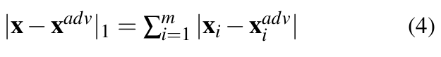
 - L1 distance (Manhattan distance): From Equation 3, L1 dis- tance can be expressed as:
- L2 distance (Euclidean distance): As per Equation 3, the Euclidean distance between x and is given by:
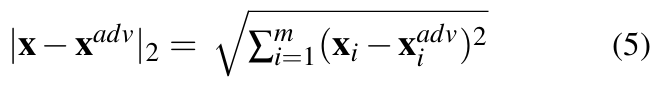
L2 can remain small even where there are minute changes in many pixels [27].
- L∞ distance (Chebyshev distance): This is given by:

Thus, L∞ measures the largest change in pixel values. This can be used to set a maximum limit up to which a pixel value is allowed to change. While any number of pixels can be modified, each pixel can only be modified to this limit.
3.3. Adversarial Examples
Adversarial examples are generated by adding computed pertur- bations to a clean image, resulting in distorted samples that look almost identical to the original image to human observers, but cause significant changes in the output class probabilities of a classifier, leading to a misclassification in majority of cases [2, 4, 25, 28]. Adversarial samples are crafted at test time and do not require an adversary to have any kind of influence on the training process [29, 30].
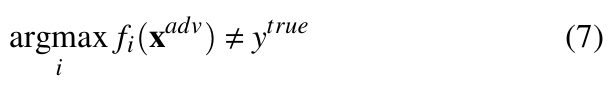
If ytrue be the true label corresponding to a clean image x, then from Equation 2 we have: argmaxi fi(x) = ytrue. If a perturbation vector η ∈ Rm is added to input x, resulting in a perturbed example xadv causing successful misclassification, then:
It is also worth noting that not all adversarial examples cause misclassification. These samples have high probability of causing misclassification but do not guarantee misclassification [25]. In this view, all samples created from an adversarial examples generation algorithm are adversarial examples but it is possible that not all of them are successful in fooling a network.
A DNN learns by iteratively reducing loss by utilizing optimization algorithms like the gradient descent. In other words, a network is made to converge to a point where the parameters are such that the resulting class probabilities yield low loss. With this in mind, the basic concept behind generating adversarial samples is to increase the loss such that the class probabilities are manipulated in a way desired by the adversary. Since it is not possible to modify the network parameters θ at test time, the input itself is varied till the goal of misclassification is met. Thus, for generating adversarial examples, the optimization problem becomes:
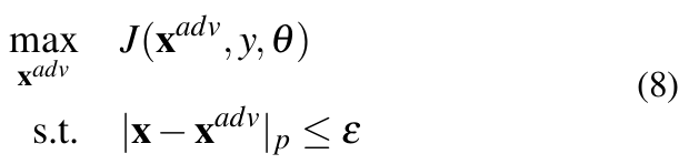
Where, ![]() = x + η and ε is the maximum allowed perturbation measured in terms of | · |p utilized by the algorithm to generate the sample.
= x + η and ε is the maximum allowed perturbation measured in terms of | · |p utilized by the algorithm to generate the sample.
3.4. Crafting Algorithms
Inducing misclassification through random perturbations is notably more challenging [23] and therefore definite algorithms are required to compute perturbation vectors of specific magnitude and direction. Usually, these algorithms aim to solve the optimization problem in Equation 8. In our original work [1], we considered five conceptually different algorithms to create such attacks. In this work, we use the same algorithms as we want to study the attack efficiency of these attacks on the source network.
Fast Gradient Sign Method (FGSM) [4]: The attack is based on the reasoning that all non-linear models are trained to behave rather linearly to make the training process easier. For instance, commonly used activation functions like ReLU are piecewise linear and even sigmoid functions are tuned to work within the linear part of the curve. As a consequence, adding linear perturbations to the input can break the models.
If perturbation vector η be the distortion introduced to input vector x such that ![]() = x + η. For |η|∞ < ε, where ε is less than the precision of the model, the model should not respond to this distortion. However, for a linear model with weight vector w, this distortion grows by w · η as shown by the relation in Equation 9.
= x + η. For |η|∞ < ε, where ε is less than the precision of the model, the model should not respond to this distortion. However, for a linear model with weight vector w, this distortion grows by w · η as shown by the relation in Equation 9.
To maximize the effect of this distortion, direction of max-norm constrained perturbation η can be aligned with weight vector. Then, m being the average weight of each element of w and n be the dimen- sion of w, the activation change can be represented as in Equation 10
The consequences of Equation 10 are: (a) Keeping the average weight same, change in activation due to η grows linearly with n. Thus, a small change at input can aggregate to create large change in output at high dimensions. (b) Since all models behave linearly, the concept of this linear perturbation can also be applied to DNNs to cause misclassifications.
Authors then use these ideas to propose FGSM which adds linear distortion to the input in a single step to create adversarial samples. The perturbation vector η is constructed as:

Thus, the adversarially perturbed sample is given by:

As can be seen, the perturbation is added in the direction of the loss gradient computed with respect to input x. This makes sense because loss gradient gives the direction of the largest increase in loss. Thus, perturbation aligned with this direction is optimal for increasing loss. ε is the L∞ norm of the perturbation which also gives the distance between x and ![]() .
.
Jacobian Saliency Map based Attack (JSMA) [29]: The attack generates adversarial examples by establishing a direct relationship between input variations and output changes, allowing it to identify the features most effective in altering the classifier’s decision.
The basic idea behind the algorithm can be summed up in three steps:
- Compute forward derivative of the function learned by the network to create a mapping between rate of change in output with respect to change in input.
- Create a saliency map based on the computed forward derivative to search for the most sensitive features that produce change towards the adversarial class.
- Add defined perturbation to the selected features. Keep adding changes iteratively with each iteration computing the forward derivative and the saliency map until the misclassification is achieved.
The forward derivative of a network computes how much the output y changes due to the change in x. Since a network learns a vector valued function, the forward derivative has to compute change in each element of y due to change in each element in x. This is basically the Jacobian of the vector valued function learned by the network.
Thus, the forward derivative is given by:
For more clarity, when assuming a 2-dimensional input x and output y, the forward derivative is computed as:

In the Jacobian matrix, a positive rate of change of an output class means that the change in the corresponding input feature will increase its current prediction probability, while a decrease means that it will decrease its prediction probability. Based on this, a saliency map can be constructed which filters the features that are most important based on the given criteria. Equation 15 provides a very basic filter criteria as defined in [29].

Here, t is the target class to which the input is to be misclassified, that is, t ≠ ytrue. S(∇ f (x), t)[i] is the saliency map computed for ith feature.
Thus, as per Equation 15, from the Jacobian matrix, features that increase the target class probability and at the same time de- crease the probabilities of all other classes are weighed. The feature with the highest value is then selected. In each iteration, selected feature is perturbed by a defined amount. This is continued till misclassification is achieved, that is, argmaxi fi(x) = t.
In practice, saliency map criteria as defined in Equation 15 is too restricting; thus, an optimized version which selects a pair of features in one iteration is often used [29]. The policy for gen- erating maps may need to be optimized as per requirement. For instance, pairwise selection is usable for CIFAR10 [31] and MNIST [32] datasets but was found to not work for datasets that contain high-resolution images like the ImageNet [27].
Universal Adversarial Perturbation (UAP) [3]: UAP is dif- ferent from other attacks discussed in this section as it generates image-agnostic perturbations. Instead of computing adversarial images for each image in a dataset, the algorithm aims to find a single perturbation vector from a given subset of data which can then be applied to the entire data distribution to create adversarial samples. These types of perturbations are called Universal Adver- sarial Perturbations (UAP). The prefix universal is used because they are generalizable across new data points that were not used when creating the perturbation.
If X = {x1, x2, . . . , xn} be a dataset sampled from a data distribu- tion µ, then the goal is to compute a universal perturbation v ∈ Rm using X, such that for most x ∈ Rm in µ, Equation 16 is fulfilled.
The algorithm iterates though each image in X and computes a perturbation vector ∆vk that sends the current data point xk + v across the decision boundary. Perturbation v is then updated as (v + ∆vk).
The perturbation vector v is such that |v|p < ξ , where | · |p is the desired Lp-norm. To make sure that the magnitude of perturbation v is within ξ , updated v is again projected onto a Lp ball of radius ξ centered at 0. The algorithm stops when a pre-defined fooling rate is obtained on X. If δ be the desired accuracy on X then the required fooling rate is denoted by (1 − δ ).
At the end of each iteration, the computed perturbation v is added to all data points in X to create a set of perturbed data points Xv = {x1 + v, x2 + v, . . . , xn + v} . The current fooling rate is then given by Equation 17. The algorithm stops when Err(xv) ≥ (1 − δ ).

The individual image perturbation ∆vk can be computed using any algorithm. For instance, authors in [3] use DeepFool [33], while [34] uses Projected Gradient Descent (PGD) [35]. In our case, we use FGSM to compute this vector and measure ξ in L∞.
The Carlini-Wagner (CW) Attack [27]: Carlini and Wagner introduce three variants of one of the most powerful gradient-based adversarial attacks against neural networks. The attacks not only cause misclassification with high success rate but they do so while introducing comparatively low distortion than other attacks like FGSM and JSMA. The three variations of the attacks are based on the L2, L0, and L∞ distance metrics. However, as in our previous work [1], we only focus on the L2 version as it is considered to be the strongest [27].
The effectiveness of the attack can be attributed to the optimization problem (Equation 18) that balances two objectives: (1) Minimize distance between adversarial and the original image. (2) Misclassify the image into any class other than the original. This results in adversarial samples that are minimally perturbed while ensuring misclassification.
In equation 18, Zi(![]() ) is the logit corresponding to the true label and Zt(
) is the logit corresponding to the true label and Zt(![]() ) corresponds to any other label t ≠ i. The equation considers L2 norm. The amount of distortion or the misclassification confidence can be controlled by varying κ. Larger κ means samples are more stronger (high confidence misclassification) at the cost of higher distortions. On the other hand, c is a positive constant that mediates the trade-off between minimizing perturbation and achieving misclassification. It is determined via binary search during the attack.
) corresponds to any other label t ≠ i. The equation considers L2 norm. The amount of distortion or the misclassification confidence can be controlled by varying κ. Larger κ means samples are more stronger (high confidence misclassification) at the cost of higher distortions. On the other hand, c is a positive constant that mediates the trade-off between minimizing perturbation and achieving misclassification. It is determined via binary search during the attack.
Further, the attack considers logits rather than activation values from the softmax layer, this enables the attack to still be effective on networks that apply gradient-masking techniques like the defensive distillation [36]. Moreover, the original paper designs the attack for targeted misclassifications, adapting the objective function accordingly. In this work, we focus on untargeted misclassification and therefore utilize the objective function presented in Equation 18.
The Boundary Attack (BA) [26]: The Attack uses model’s decisions on the input points to craft adversarial examples and there- fore, unlike other attacks discussed in this section, it does not require access to model parameters or architecture to create adversarial samples.
For each clean image, the algorithm initializes a random adversarial image and iteratively applies perturbations that reduce the L2 distance between the adversarial and the corresponding clean image. After each iteration, the algorithm checks that the perturbed image remains outside the decision boundary of the original image by querying the model. This process continues until the minimum distance between the clean and adversarial image is achieved.
The algorithm internally uses two parameters, δ and ε to control the perturbations that guide the initialized image towards the clean image. δ controls the magnitude of the perturbations and ε controls the step size towards the clean image. The generation process begins by sampling feature values from a uniform distribution U (0, 1) to create a random image that is adversarial to the clean image. Multiple perturbations are sampled randomly from an iid Gaussian distribution N (0, 1) and are rescaled based on the current value of δ . These perturbations are then projected on a sphere around the clean image and are then added to the random image. From the resulting perturbed images, only those that are still adversarial are selected for further processing. If less than 20% of the perturbed images are adversarial, then this means that the image is already close to the decision boundary, and thus the value of δ is decreased. However, if more than 50% are adversarial, then δ is increased. Finally, to make a movement towards the decision boundary, the perturbations are again scaled by ε and added to the perturbed images. Again, out of the resulting perturbed images, only those that remain adversarial are selected. Value of ε is adjusted by considering similar thresholds as in the case of δ . From the successful adversarial images, the adversarial image that is closest to the initial image in terms of L2 distance is selected for the next iteration. The loop continues with the updated values of δ and ε until an adversarial image with minimum possible L2 is obtained. Thus, with each iteration, the adversarial image comes closer to the decision boundary and starts to look like the original image, yet remaining adversarial.
Both δ and ε are adjusted automatically during generation. The number of iterations, however, is provided as input to the algorithm.
Fewer iterations result in higher distortion, while more iterations result in less distortion, as the algorithm has more opportunities to bring the initial image closer to the original image.
Moreover, BA is a gradient-free attack as it does not use any type of gradient-information to craft adversarial samples.
3.5. Quantization as a Model Optimization Technique
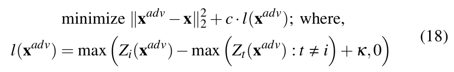
Quantization reduces the computational complexity during training and inference by reducing the bitwidth of activations, gradients, and weights [18] to lower bitwidth numbers. This allows floating- point multiplications during convolution operations to be replaced with faster bitwise operations. For instance, by binarizing weights and input activations of convolution layers, the dot products during forward pass can be computed with the formula as in Equation 19 [37].

Here, x and y are two bit vectors and the bitcount operation counts the number of 1s in the resulting vector. Equation 19 can be further extended to be valid for any fixed-point integer values.
If x be a sequence of M-bit integers and y be a sequence of K-bit integers then:
where, ![]() are bit vectors bit vectors. Then the dot product of x and y is given by Equation 22 [37].
are bit vectors bit vectors. Then the dot product of x and y is given by Equation 22 [37].
Thus, by representing activation, weights, and gradients by integer values, convolution operations between them can be greatly optimized.
There are two types of quantization [20, 22]: post-training quantization and quantization aware training. In post-training quantization, weights and activation values are quantized after a model is fully trained. Quantization aware training quantizes weights, activations, or gradients during training.
DoReFa-Net [37]: The quantization method quantizes weights, activations, and gradients to lower bitwidths during training. Activation and weight values are quantized during forward pass, while the gradients are quantized during backward pass. Although DoReFa- Net is able to perform low bitwidth quantization of gradients, we do not consider gradient quantization in this work. Thus, the convolution operation between weights and activations during forward pass takes place in low bitwidths, while backward pass still requires convolution between quantized and unquantized values.
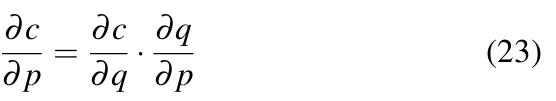
If q is a quantized value of p and c is the cost function, then during backward pass, computation as in Equation 23 requires ![]() which is not well defined. This creates a problem during backpropagation.
which is not well defined. This creates a problem during backpropagation.
One of the solution to this problem is to estimate the value of ![]() , given that
, given that ![]() is properly defined. These estimators that allow defining custom
is properly defined. These estimators that allow defining custom ![]() are called Straight Through Estimators or STEs [38]. DoReFa-Net uses quantizen STE [37], which is defined as in Equation 24.
are called Straight Through Estimators or STEs [38]. DoReFa-Net uses quantizen STE [37], which is defined as in Equation 24.
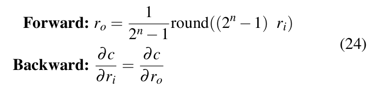
Equation 24 uses ![]() as an approximate of
as an approximate of ![]() .In the equation, ri ∈ [0, 1] is a float32 real number and ro ∈ [0, 1] is the quantized output value representable by an n-bit number. Since there is always an affine mapping between fixed-point integers and n-bit numbers, the bit-convolutions as specified in Equation 22 can take place be- tween quantized weights and activations during forward pass. This significantly speeds-up the training and inference process.
.In the equation, ri ∈ [0, 1] is a float32 real number and ro ∈ [0, 1] is the quantized output value representable by an n-bit number. Since there is always an affine mapping between fixed-point integers and n-bit numbers, the bit-convolutions as specified in Equation 22 can take place be- tween quantized weights and activations during forward pass. This significantly speeds-up the training and inference process.
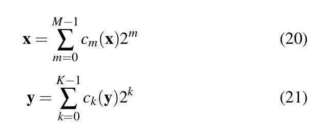
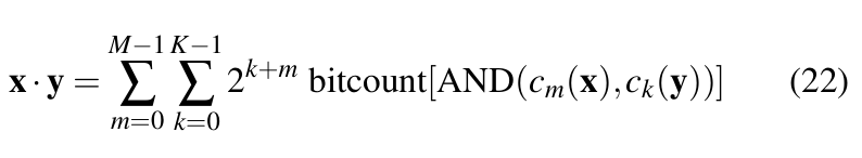
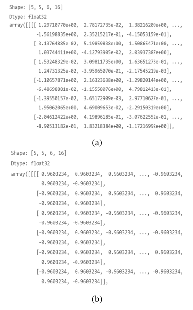
Figure 1 compares weight values of a convolution layer before and after 1-bit quantization using DoReFa-Net. As illustrated in the figure, the weight values are 1-bit quantized (2 possible values) but the data type remains float32. We maintain the n-bit numbers as float32 and do not convert them to integers. This approach preserves the levelling effect caused due to quantization, but without the speed optimizations that integer representations could provide. However, improving computational speed is not a priority, as the primary goal is to analyze the network’s behaviour.
Quantization of weights: DoReFa-Net treats 1-bit quantization of weights differently than n-bit quantization where n > 1. For 1-bit quantization, a method similar to [39] is used. The STE is as shown in Equation 25.
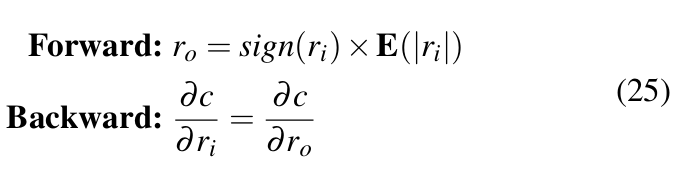
Here, ![]() has two possible values: -1 and 1. E(|ri|) is the average of absolute values of all weights in the layer. For n-bit quantization, forward operation as in Equation 26 is used.
has two possible values: -1 and 1. E(|ri|) is the average of absolute values of all weights in the layer. For n-bit quantization, forward operation as in Equation 26 is used.

Here, tanh bounds the value of ri within [-1,1]. The expression 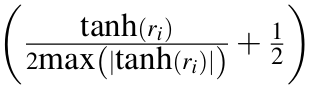 results in a value between [0,1], maximum here is taken over all weights in that layer.
 ![]() thus quantizes weights to n-bit numbers within [-1,1].
thus quantizes weights to n-bit numbers within [-1,1].
Quantization of activations: The input to each weight layer is quantized with forward operation as defined in Equation 27.

Here, ri is passed through an activation function that limits it within [0,1] before being used as input to ![]() .
.
4. Related Work
In our previous work [1], we performed a comprehensive analysis of transferability among quantized and full-precision networks trained on the MNIST and CIFAR-10 datasets. The analysis involved various attack algorithms, as well as variations in model-related properties like architecture and capacity. The findings show that although transferability, in general, remains poor, it may be possible to improve the attack transfer rate using UAP. Further, it was observed that the attacks like BA and CW had high efficiency when applied on the source network even in the case of low-bitwidth networks. Additionally, it was observed that an attacker might be able to predict the success rate of an attack on a target network with different bitwidths, capacities, and architectures based on the per- formance of the attack when transferred among different bitwidth versions of the source model.
There has been substantial research related to network quantization, adversarial examples, and the impact of adversarial attacks on both full-precision and quantized models, providing significant insights into the vulnerability and robustness of quantized networks.
4.1. Quantization
A survey on various works on quantization of DNNs is presented in [20]. The paper provides an overview of different types and techniques of quantization along with the references to different networks that implement those methods. The case studies presented in the paper involving XNOR-Net [39] and Binaryconnect [40] provide a good starting point for understanding binarized networks. The paper also provides an introduction to the DoReFa-Net method [37] which is used in this work for quantization. Further, it also compares DoReFa-Net with other quantization methods in terms of accuracy of the resulting quantized networks. The comparisons in this paper helped to confirm that DoReFa-Net had no known issues and that the performance was comparable, if not better, than other similar quantization techniques. This strong performance was a key factor in our decision to select DoReFa-Net for quantization.
Authors in [18] provide details on how TensorFlow Lite [41] can be used for quantization. Although the strategies and the quantization process itself are only focused on TensorFlow Lite’s implementation, the findings are significant and can be generalized for other quantization tools as well. The key takeaway is that fine-tuning an already trained network leads to better accuracy models after quantization than training from scratch and that the models with large number of parameters are more resistive to accuracy loss due to quantization. This observation is in agreement with the conclusion drawn from the model configuration experiment in [37].
In [42], authors present an open-source model optimization framework called Mayo which supports multiple compression techniques like the Low-rank Approximation (LRA) [43], quantization and pruning [17]. These compression techniques are implemented through objects called overriders which can be applied to any net- work component like weights, biases, activations or gradients to customize their value. Further, Mayo also allows chaining of multiple overriders meaning that multiple compression techniques can be applied in a sequence. This unique ability enables Mayo to achieve higher compression ratio than any other compression APIs.
However, there are several drawbacks with Mayo; for instance, it uses multiple YAML files for configuration, which makes it customizable but also makes the control flow complex and hard to comprehend for custom implementations. Moreover, there is no clear explanation on how quantization is performed. Authors mention that the quantization is fixed point [42] but do not go into details on how this is done.
The Model Optimization Toolkit2 from TensorFlow provides multiple methodologies for network quantization. However, the post-training quantization does not support quantization other than 16-bit float and 8-bit integer. The quantization aware training allows to define specific bitwidths for each layer during training, but quantization parameter configuration (like custom bitwidths) are not supported for deployment, meaning that although network layers can be trained at lower bitwidths, model execution takes place at 8 bits. Therefore, lower bitwidth quantization is not possible.
4.2. Adversarial Examples
In [4], authors argue that adversarial examples exist not due to extreme non-linearity or over-fitting of a model, but rather because of its linear behaviour in high dimensions. Authors use this hypothesis to introduce the Fast Gradient Sign Method (FGSM) for creating adversarial examples. FGSM being able to produce successful adversarial examples provides validity to the claim that these examples exploit the model’s inherent linearity. The paper also makes an important observation that the adversarial examples exist in broad contiguous regions in input space rather than in fine pockets. For multiple models, these adversarial subspaces are shared. Perturbations leading to the shared subspaces lead to adversarial transfers. Thus, direction of perturbation is important for transferability rather than magnitude.
Authors further explore the concept of adversarial subspaces in [23] where they estimate the dimensionality of this subspace. They find that compared to the input dimension, the dimension of the adversarial subspace is relatively small. The perturbation directions leading to the adversarial subspace are referred to as adversarial directions. These orthogonal adversarial directions are shared across multiple models, forming a common subspace. As a result, all adversarial points within this shared subspace are transferable, meaning they can fool any model that share it. Further, authors show that the minimum distance required to cross the decision boundary for any data point is least in the adversarial direction while it is higher in random directions. This means that adding small perturbations is enough to make the data point cross the decision boundary if the perturbation is in the adversarial direction, while larger perturbations are necessary if the perturbation directions are random.
A comprehensive study on how model-specific properties like model accuracy, capacity, and architecture affect transferability is presented in [24]. Here, the authors use Iterative Fast Gradient Sign Method (IFGSM) [25] and FGSM to generate adversarial attacks; hence, the findings are valid only for attacks that leverage loss gradients to create adversarial samples. Authors show that the attacks crafted on low-accuracy networks have very poor transferability regardless of model’s capacity and that same architecture transfers are better than different architecture transfers. Further, authors argue that the iterative attacks transfer better than single-step attacks; however, direct attack effectiveness is not considered.
In [30], authors use a custom attack based on Projected Gradient Descent (PGD) algorithm [35] to study both transferability and direct attack effectiveness on various types of networks. Different types of classifiers including Support Vector Machines (SVMs), logistic regression, and neural networks are considered. Authors find that high-complexity networks require less distortion to produce successful adversarial examples because sudden changes in the loss function mean local optima are easier to find. This also meant that highly regularized models were hard to create successful adversarial samples against. Moreover, authors also find that both transferability and attack performance on the source network increases when the hyperparameter value associated with the attack is increased. However, since the attack is gradient-based, the observations, like [24], are limited for gradient-based attacks.
The study in [44] offers a unique perspective on adversarial examples, arguing that all datasets contain non-robust features which are imperceptible to humans but are highly predictive. Models become sensitive to these features as they learn to rely on them during training. These features are brittle and therefore samples with slight change in them can cause misclassification. Additionally, these features being non-perceptible also means that changes are not visible. The presence of these non-robust features also leads to adversarial examples being transferable because all datasets contain these features and thus models trained on similar datasets are likely to learn similar non-robust features.
In [45], authors present a study on transferability among multiple networks. The paper considers various models including ResNet50, ResNet101, ResNet152, VGG16, and GoogleNet [46]. FGSM, FGM (Fast Gradient Method), and a custom optimization based attack3 are used to generate adversarial examples. Both FGM and optimization based attack were found to have similar transferability. Interestingly, the transferability between networks with similar architectures was not found to be consistently better than between networks with different architectures, a result that contrasts with [24] but aligns with our findings in [1]. Moreover, the authors observed that the optimization based attack performed better than the other two attacks when applied on the source network, possibly because FGSM and FGM create adversarial samples in a single step and thus sacrifice efficiency for speed.
Authors in [47] use a tool called Deep Learning Verifier (DLV) [48] to generate adversarial examples. DLV performs an exhaustive search within a defined radius around an image and returns all possible adversarial examples (if any) and thus provides a guarantee that apart from the ones that are discovered, the image is robust against all other perturbations within the defined region. In their experiments, authors find that some classes in MNIST dataset had smaller number of effective adversarial samples than others. This indicates that not all classes in a dataset are equally robust and some might be more vulnerable than others.
Regarding adversarial attack generation, there are several popular tools that can be used to implement multiple attack algorithms. For instance, [26] uses FoolBox [49] to implement FGSM and DeepFool [33] attacks; [27] and [23] uses CleverHans library [50] to implement JSMA and FGM, respectively. Moreover, several works like UAP provide open source access to their work4 so that the community can build on them. In [1] and in this work, we use Adversarial Robustness Toolbox (ART) [51] to create adversarial examples. The library supports comparatively large number of attack algorithms and provides comprehensive documentation for each attack implementation, along with an actively maintained codebase5.
4.3. Vulnerability of Quantized Networks to Adversarial Examples
In [22], authors use multiple attack algorithms to evaluate the robustness of quantized networks against adversarial attacks. The paper uses DoReFa-Net for network quantization. However, Binary Neural Network (BNN) [52] is used for 1-bit quantization while DoReFa-Net is used only for 2-bit, 3-bit, and 4-bit quantization. The robustness of quantized networks against attacks created on the same network as well as against transfer-based attacks is examined for five attack types: FGSM, Basic Iterative Method (BIM) [25], Simultaneous Perturbation Stochastic Approximation (SPSA) [53], CW attack, and Zeroth Order Optimization (ZOO) [54]. Authors observe that gradient masking caused by activation quantization may increase the robustness of a quantized network against gradient- estimation algorithms like ZOO and gradient-based attacks like FGSM and BIM, but some gradient-estimation algorithms, like SPSA and CW, that are specialized to handle noise function were found to be still effective. These observations are similar to ours as we discuss in Section 7.2. However, we analyse this phenomena further with additional attacks. Furthermore, authors show that weight-only quantization does not affect attack performance at source as the attacks can still produce similar variance in logit values in quantized networks as in full-precision networks.
The work in [21] investigates the transferability of adversarial attacks among compressed networks. The study considers pruning and quantization as compression techniques and uses Mayo [42] for compression. BIM, IFGM, and DeepFool are used to craft adversarial examples. Authors show that the density of a network can be reduced to as low as 15% for both CIFAR10 and MNIST networks without any reduction in the test accuracy. This is inter- esting because it shows that majority of parameters in a network are not significant and supports the claim in [20] that low-bitwidth quantization works because most parameters in a network are not useful.
Authors in [34] present a transferability study that implements various compression techniques including quantization to analyse the transferability of the UAP attack across compressed networks. A method called Additive Powers-of-two (APoT) [55] is used for quantization. PGD is used to create UAPs. The difference between the UAP crafted using PGD and FGSM (as used in this work) is that the PGD updates the overall noise vector v in mini-batches, while FGSM updates it per image. An important observation is that SVHN dataset [56] was found to be more robust against attacks created and applied on the same network as compared to CIFAR10 even when both CIFAR10 and SVHN were trained on the same network and images in both datasets had the same resolution. This indicates that some datasets are more robust to adversarial attacks due to the nature of data. Further, similar to [22], authors argue that quantization can cause gradient-based attacks to perform poorly on the source network due to gradient masking. Experiments in the paper also show that transferability is poor when source and target networks differ in bitwidths, as well as when they differ in the type of compression algorithm used.
5. Adversarial Neural Network Toolbox (ANNT)
We introduce Adversarial Neural Network Toolbox (ANNT) [57], an open-source tool that provides a unified interface for handling the complete workflow of quantized model training, adversarial image creation, and model robustness evaluation. Figure 2 shows the usability of the tool in terms a basic workflow.
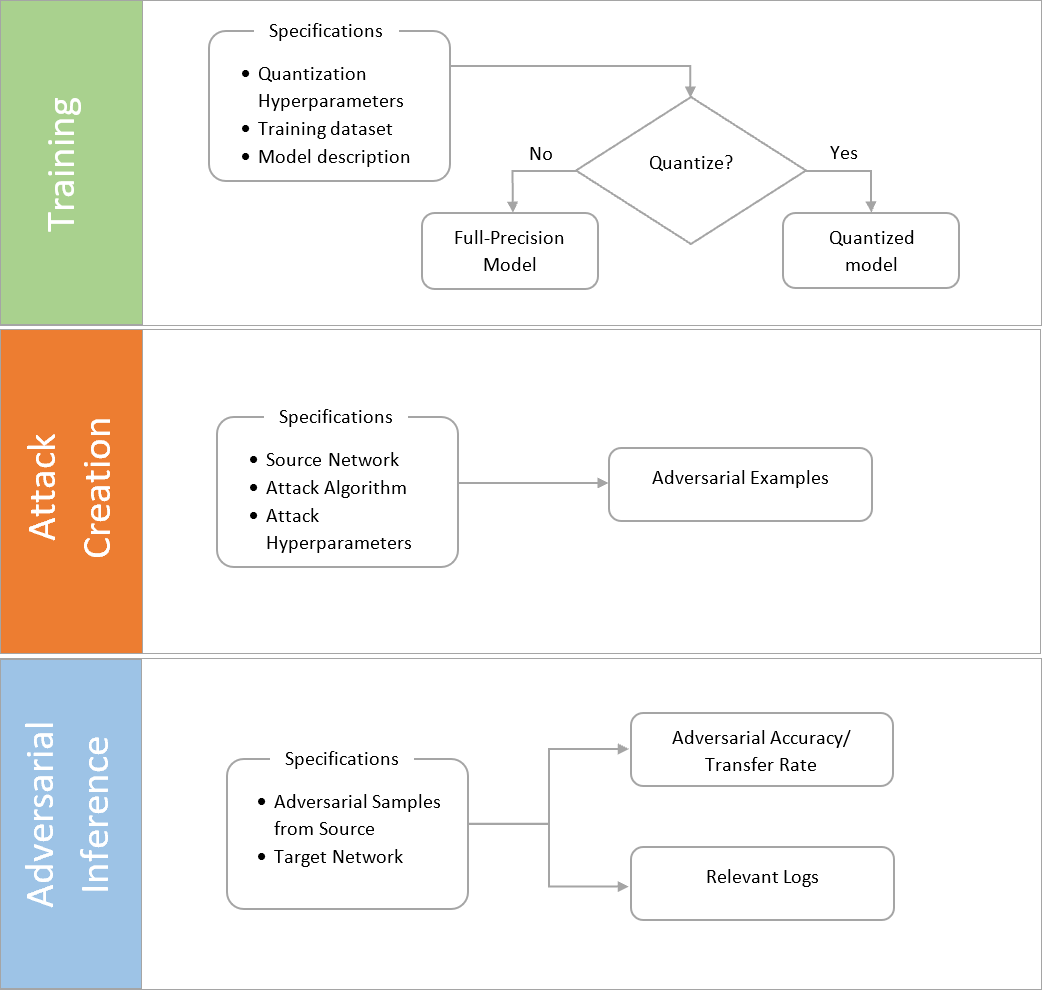
To train full-precision models, users can provide the model description (architecture), input dataset, and training hyperparameters. Additionally, quantization hyperparameters such as the weight, activation, and gradient bitwidths can be provided to train quantized versions of a network.
The tool provides a unique functionality of generating adversarial examples on a network of specified bitwidth. Users can provide a trained model, quantization bitwidth, adversarial attack algorithm, and attack hyperparameters to create specified number of adversarial samples.
Further, the tool can also be used to perform adversarial inferences on any given target network. The process computes the accuracy of the target network against the input adversarial samples. It also generates other relevant information like the correctly and incorrectly classified samples and average L∞ and L2 distance between the successful adversarial and clean samples. Thus, the cumulative information generated is enough to perform a comprehensive analysis of both direct and transfer-based attacks.
The tool can be used as a standalone Python application or as a library. When used as an application, configurations like current task (training/ inference/ attack creation), bitwidths, adversarial attack algorithm (for attack creation), training hyperparameters, and dataset can be provided through a YAML file. The tool then ex- ecutes the specified task and provides detailed logs of the entire process. When used as a Python library, users can simply import ANNT as a module and utilize the provided interfaces for each task. Additionally, an interface to load the generated samples for visualization is also included. The repository provides a detailed wiki as well as sample notebooks to help users get started with the tool.
In addition to MNIST trained LeNet-5 [32] and CIFAR10 trained Resnets [15] of different capacities including Resnet20, Resnet32, and Resnet44, several custom Convolutional Neural Net- works (CNNs) trained on MNIST and CIFAR10 are supported out- of-the-box. Further, five different attack types—FGSM, CW attack, Boundary Attack, JSMA, and UAP—are supported.
The tool is based on TensorFlow 1.13 [58] and uses Tensorpack 0.11 [59] for model training and inference. Further, DoReFa-Net [37] is used for quantization while Adversarial Robustness Toolbox (ART) [51] is used to create adversarial samples.
6. Experimental Setup
6.1. Datasets and Models
The details regarding the datasets and full-precision (32-bit) models used in the experiments are shown in Tables 1 and 2, respectively.
Table 1: MNIST and CIFAR10 datasets.
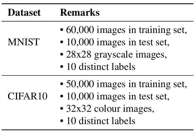
Table 2: Full-precision (FP) MNIST and CIFAR10 models used in the experiments.
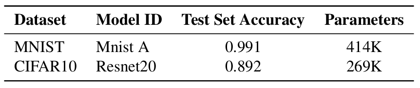
All models were trained from scratch. The MNIST model (named as Mnist A) is a custom CNN while Resnet20 is a ResNet [15] trained on CIFAR10. The model architecture for Mnist A6 and Resnet207 are based on the examples defined in the Tensorpack repository [59].
6.2. Quantization
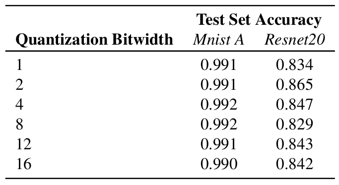
1-bit, 2-bit, 4-bit, 8-bit, 12-bit, and 16-bit quantized versions of the models in Table 2 were trained. As recommended in [37], the first and last layers were not quantized in favour of better accuracy.
Quantization here refers to weight and activation quantization. Thus, an 8-bit network means both weights and activations are quantized to 8 bits.
Table 3 shows the accuracy of the quantized versions of the Mnist A and Resnet20 models. Like the FP versions, all quantized models were trained from scratch. As can be seen, quantization did not result in noticeable drop in accuracy for models trained on MNIST, while CIFAR10 models show a non-negligible decrease in accuracy. This was expected because DoReFa-Net is known to result in accuracy drops for more natural datasets [37].
Table 3: Test set accuracy of the quantized versions of the Mnist A and Resnet20.
6.3. Attacks and Metrics
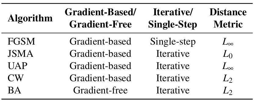
Attacks: Table 4 summarizes the attack algorithms used along with other relevant information.
Table 4: Adversarial attack algorithms used and their key characteristics.
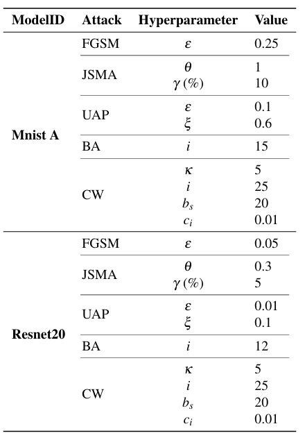
Attack hyperparameters: Table 5 shows the selected hyperparameter values for each attack type for both Mnist A and Resnet20 models.
In the case of FGSM, ε controls the magnitude of perturbation introduced to the images. In JSMA, θ is the amount of distortion added per feature in each iteration and γ is the percentage of features allowed to be distorted for an image. For UAP, ε is the perturbation magnitude for FGSM which is used to generate adversarial examples within the UAP (Section 3.4), ξ is the maximum allowed magnitude of perturbation of the UAP noise vector. As recommended in [34], we measure ξ in L∞. For the Boundary Attack, i is the maximum number of iterations8. Finally, for CW attack, κ ≥ 0 controls attack confidence, i is the number of iteration the algorithm runs per image (gradient descent steps), c > 0 is a balancing constant used in the optimization problem (Equation 18), bs is the number of binary search steps to determine c, and ci is the initial value of c. The values of ci and bs were selected based on the original paper [27], while κ was varied to control distortion. The values of hyperparameters in Table 5 were selected such that the images were distorted but yet remained recognizable to human observers.
Table 5: Attack hyperparameter values for the full-precision (FP) and quantized versions of the MNIST and CIFAR10 models.
Attack metrics: Based on the metrics used by the current state of the art, there are two possibilities for representing the effective- ness of an adversarial attack on a network: adversarial accuracy and evasion rate.
Adversarial Accuracy is the accuracy of a network against adversarial examples. It is expressed as the ratio of the number of adversarial examples that are classified correctly by the network to the total number of samples used to attack the network.
For a set of pairs of clean sample and its adversarial counterpart,
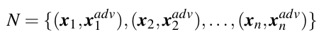
the adversarial accuracy is computed as below:
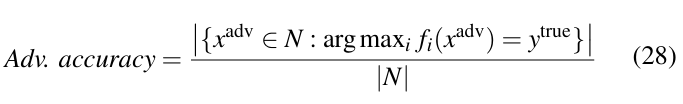
Here, f is the classifier in which the attack is applied.
Similarly, evasion rate gives the success rate of the adversarial attack on a network. It is defined by the ratio of the number of adversarial examples that are classified incorrectly by the network to the total number of samples used to attack the network. This is computed as:
A network having higher adversarial accuracy means the model is more robust against the attack, while an attack having higher evasion rate means the network is less robust.
Any one of these metrics can be used to represent adversarial robustness. [21, 22, 45] use Equation 28, whereas [23, 24, 30, 34] use Equation 29.
In this paper, we use adversarial accuracy, as we have selected the same metric in [1]. This is simply a preference, using evasion rate would not affect the observations or the results.
Training of all models, adversarial examples creation, and computation of adversarial accuracy on target network were done using ANNT.
7. Experiments, Observations, and Analysis
7.1. Experiments
A random sample of 1,000 clean images was selected from the MNIST dataset (Table 1). Taking FP Mnist A (Table 2), and its quantized counterparts (Table 3) as source networks, adversarial examples were created using all attack types described in Table 4 with attack hyperparameter values as described in Table 5. When creating adversarial examples, inherent inefficiencies of the models were avoided by selecting only those clean samples that were correctly classified by the source network. The samples were then applied on the same source network. The resulting adversarial accuracy of the network, along with the average L2 and L∞ distances (as a measure of distortion) between the successful adversarial and clean samples were recorded. The samples were taken again, and the process was repeated for 3 independent runs.
The same procedure was performed for FP Resnet20 (Table 2) and its quantized versions (Table 3). Table 6 shows averaged adversarial accuracies and the Lp distances from the 3 runs for each MNIST and CIFAR10 model.
7.2. Observations and Evaluation
Based on the results in Table 6, the following observations can be made:
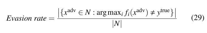
Observation 1: The Boundary Attack has high effectiveness. For both CIFAR10 and MNIST models, the Boundary Attack shows very high effectiveness while requiring very less number of iterations to look like the original image. From Figure 3, it can be seen that it just takes about 15 iterations for MNIST and 12 for CIFAR10 for the adversarial images to look like the original image. This also goes along with the observation made in [26] where it takes very less number of iterations to make the initial random image look like the original image with more visible distortions at lower iterations. The attack’s high effectiveness across all models, including the quantized ones, makes sense because it keeps the initialized image adversarial for any number of iterations in all cases.
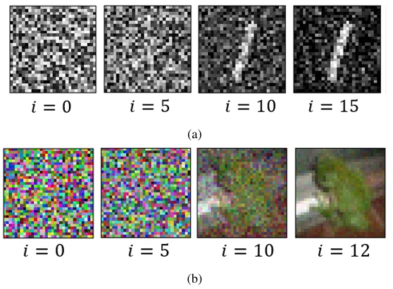
Observation 1.1: Adversarial images generated by the Boundary Attack are more distorted in case of quantized networks. Ideally, when given enough iterations, the Boundary Attack should generate adversarial image which looks exactly like the original image with no visible distortions. However, compared to the FP models, majority of the adversarial images produced with quantized models especially at lower bitwidths were more distorted. This can also be observed in terms of L2 distances in Table 6 where L2 distances in case of 1-bit quantized network is higher when compared to the corresponding FP network.
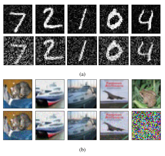
Figure 4 shows a comparison between adversarial images gen- erated from the FP and 1-bit quantized models. As can be seen, the adversarial images for 1-bit models are more distorted with one of the images in the quantized version of Resnet20 being non- recognizable (elaboration in observation 1.2). It can be hypothesized that this is because quantized networks are more resistive to noises in the input data than their FP counterparts. The activation quantization causes activation values to be clipped [21] because of which it
Table 6: The adversarial accuracy of FP and quantized versions of Mnist A and Resnet20 against the five attacks. Attacks were created and applied on the same network. The average L2 and L∞ distances between the successful adversarial example and the corresponding clean sample is shown as well.
| Mnist A | ResNet20 | |||||||
| Bitwidth Attacks | Hyperparameter
Values |
Adversarial
Accuracy |
L2 | L∞ | Hyperparameter
Values |
Adversarial
Accuracy |
L2 | L∞ |
| FP | 0.337 | 5.219 | 0.25 | 0.119 | 2.740 | 0.05 | |||||
| 1 | 0.845 | 5.134 | 0.25 | 0.137 | 2.737 | 0.05 | |||||
| 2 | 0.750 | 5.116 | 0.25 | 0.206 | 2.742 | 0.05 | |||||
| 4 | FGSM | ε | = 0.25 | 0.715 | 5.128 | 0.25 | ε | = 0.05 | 0.292 | 2.742 | 0.05 |
| 8 | 0.678 | 5.132 | 0.25 | 0.299 | 2.736 | 0.05 | |||||
| 12 | 0.493 | 5.120 | 0.25 | 0.308 | 2.736 | 0.05 | |||||
| 16 | 0.480 | 5.129 | 0.25 | 0.367 | 2.737 | 0.05 |
| FP | 0.116 | 5.436 | 1 | 0.074 | 2.425 | 0.436 | |||||
| 1 | 0.339 | 7.801 | 1 | 0.142 | 2.504 | 0.513 | |||||
| 2 | θ | = 1, | 0.375 | 6.707 | 1 | θ | = 0.3, | 0.247 | 2.581 | 0.395 | |
| 4 | JSMA | γ | = 10% | 0.140 | 6.814 | 1 | γ | = 5% | 0.419 | 2.804 | 0.484 |
| 8 | 0.064 | 5.739 | 1 | 0.351 | 2.680 | 0.505 | |||||
| 12 | 0.066 | 6.370 | 1 | 0.469 | 2.720 | 0.502 | |||||
| 16 | 0.148 | 6.981 | 1 | 0.430 | 2.808 | 0.515 |
| FP | 0.114 | 9.352 | 0.6 | 0.176 | 3.362 | 0.1 | |||||
| 1 | 0.683 | 9.073 | 0.6 | 0.110 | 3.430 | 0.1 | |||||
| 2 | ε | = 0.1, | 0.555 | 8.585 | 0.6 | ε | = 0.01, | 0.154 | 3.275 | 0.1 | |
| 4 | UAP | ξ | = 0.6 | 0.438 | 8.685 | 0.6 | ξ | = 0.1 | 0.169 | 3.414 | 0.1 |
| 8 | 0.378 | 8.648 | 0.6 | 0.192 | 3.308 | 0.1 | |||||
| 12 | 0.174 | 8.618 | 0.6 | 0.297 | 3.390 | 0.1 | |||||
| 16 | 0.162 | 8.159 | 0.6 | 0.175 | 3.275 | 0.1 |
| FP |
κ = 5, i = 25, bs = 20, ci = 0.01 |
0.037 | 3.655 | 0.888 |
κ = 5, i = 25, bs = 20, ci = 0.01 |
0.000 | 0.111 | 0.014 | |
| 1 | 0.526 | 5.220 | 0.944 | 0.000 | 0.822 | 0.104 | |||
| 2 | 0.558 | 5.047 | 0.928 | 0.000 | 0.360 | 0.049 | |||
| 4 | CW | 0.148 | 3.182 | 0.803 | 0.000 | 0.249 | 0.041 | ||
| 8 | 0.190 | 3.833 | 0.897 | 0.001 | 0.155 | 0.020 | |||
| 12 | 0.163 | 3.650 | 0.874 | 0.000 | 0.102 | 0.013 | |||
| 16 | 0.106 | 3.066 | 0.780 | 0.000 | 0.112 | 0.013 |
| FP | 0.000 | 5.507 | 0.629 | 0.000 | 2.387 | 0.155 | |||
| 1 | 0.000 | 6.259 | 0.634 | 0.012 | 2.816 | 0.184 | |||
| 2 | 0.000 | 4.649 | 0.507 | 0.066 | 2.603 | 0.170 | |||
| 4 | BA | i = 15 | 0.000 | 4.338 | 0.488 | i = 12 | 0.045 | 2.859 | 0.186 |
| 8 | 0.000 | 4.267 | 0.493 | 0.080 | 2.904 | 0.189 | |||
| 12 | 0.001 | 3.664 | 0.432 | 0.002 | 3.128 | 0.203 | |||
| 16 | 0.000 | 3.235 | 0.387 | 0.080 | 2.803 | 0.184 |
becomes hard to produce differential activations from small changes at the input9, and thus, even when the input has slight perturbations, quantized networks can correctly classify the image. This is also evident from the data from other attack types where for the same value of attack hyperparameters, FGSM, JSMA and UAP perform comparatively bad when the network is quantized. In the case of the Boundary Attack, this could mean that the algorithm cannot further reduce the distortions in an image because then the quantized network will classify the adversarial example correctly.
This hypothesis was put to test by increasing the number of iterations in the Boundary Attack to 1,000 for the 1-bit quantized Mnist A model. As can be seen in Figure 5a, the adversarial images are still equally distorted for 1-bit quantized version; whereas, the distortions are significantly less even for less number of iterations for the FP models, as seen in Figure 5b. Therefore, it would not matter if the iterations are increased any further because the algorithm will not be able to reduce the distortions due to the network being insensitive to small noises at input.
Quantized networks being more resistive to input noises is also observed in [47] and [34] where the authors find that the perturbations that worked in FP stopped working in quantized networks. Quantization thus acting as a filter for adversarial noise.
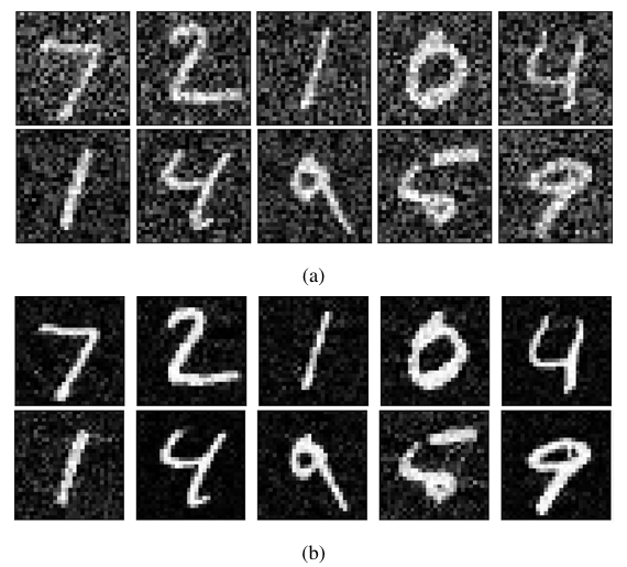
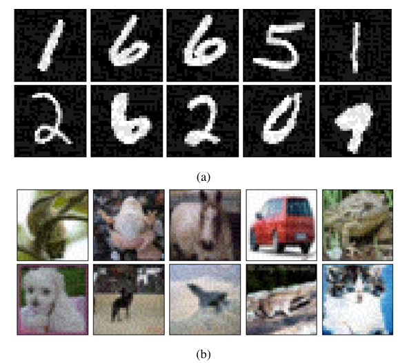
Observation 1.2: Imperceptible adversarial images resulting from the Boundary Attack on quantized networks. Apart from the images that are distorted but recognizable to human oracles, the Boundary Attack also resulted in adversarial images that were completely distorted and unrecognizable but only in case of quantized networks. Figure 6 shows adversarial images generated by the Boundary At- tack on 1-bit quantized versions of Mnist A and Resnet20 models. As can be seen, multiple images in both figures are unrecognizable. This could again be due to the algorithm not being able to re- duce the distortion any further because of the model being robust against input noises. To verify this, an experiment was performed in which adversarial examples were generated from 3,000 randomly sampled clean images from MNIST and CIFAR10 datasets using the 1-bit quantized versions of Mnist A and Resnet20 as source. The images that seemed to be composed of random pixels were then isolated and inferences were ran on them. It was found that for all of these images, the true class was within top-2 predicted classes. This indicates that the Boundary Attack could not reduce the L2 distance between the original and the adversarial image any further because any further reduction would cause the image to go inside the decision boundary of the original image making the image no longer adversarial.
Imperceptible images having true labels within top-2 predicted classes also means that although the features in the images in Figure 6 are not recognizable to human observers, the network identifies these features and tries to classify them to the correct class. These features that are non-recognizable to humans but tend to be meaningful and predictive for networks are studied in [44].
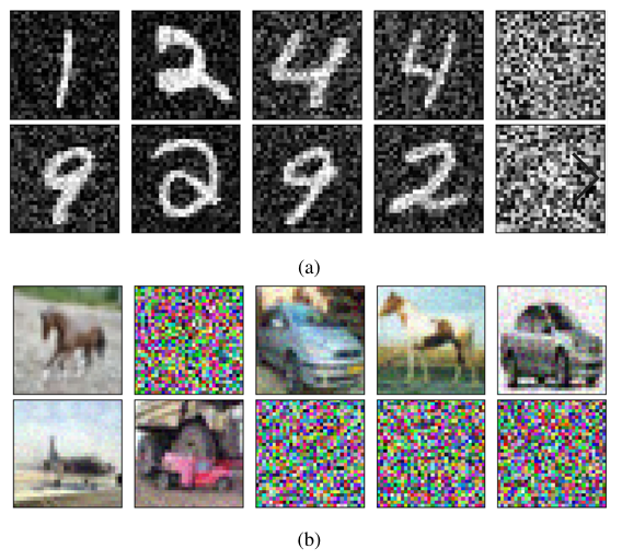
One of the important qualities of adversarial examples is that they should be classified correctly by human oracles, and since these images are completely distorted, they cannot be considered as adversarial images. Thus, these examples were removed when computing source network performance in Table 6.
It is also worth noting that these imperceptible images are rare. In a set of 3,000 random images, on 3 separate runs, for 1-bit quan- tized Resnet20 at 12 iterations, only about 280 images on average were imperceptible. Similarly, for 1-bit quantized Mnist A at 15 it- erations, on average only about 180 such images were found. Thus, these images formed very small portion of the total adversarial examples generated and only occurred for quantized networks.
The presence of these images when creating adversarial images from the Boundary Attack also suggests that although networks show near-zero resistance against the attack, quantized networks do offer certain form of resilience because valid adversarial images that have less distortion or are at least recognizable to humans become hard to create when networks are quantized.
Observation 2: CIFAR10 models require less distortion than MNIST models to produce misclassification. As can be seen from Table 6, for CIFAR10 models lower distortions are enough for the attacks to perform well, while the MNIST models require comparatively higher value of the attack hyperparameters.
There are two reasons for this. The first reason is that the MNIST dataset has less intra-class differences [26] which makes the classification problem easier to solve, and thus the network is less sensitive to small changes or perturbations [34]. However, in case of CIFAR10, a single class can have a large variety of objects of different shapes, sizes, and color, and thus a small change in any of the input features is enough to produce misclassification [34]. For instance, considering FGSM with ε = 0.1 in case of FP Mnist A model, the average adversarial accuracy from 3 separate runs on 1,000 samples was found to be 0.831. In contrast, for FP Resnet20 model, for the same attack with ε = 0.025, the average adversarial accuracy was found to be 0.127. Thus, comparatively, CIFAR10 trained network was more vulnerable to the resulting adversarial samples even in relatively low distortion. In both cases, the value of hyperparameter ε is selected such that the distortions were barely visible, as seen in Figure 7. Similar behaviour is reported in [34] with SVHN, an MNIST-like dataset, where SVHN models are more robust to UAP based attacks as compared to CIFAR10 models.
Another reason why CIFAR10 models show more vulnerability is the high-dimensionality of the CIFAR10 dataset as compared to MNIST. For Attacks like FGSM and UAP, which add a constant perturbation to the input in a specific direction, the same value of the constant introduces larger change at the output in higher dimension. This is also evident from Equation 10. Keeping ε constant and increasing n would cause larger change in the activations.
For CW attack as well, we can see that the same value of hyper- parameters are more effective in CIFAR10 models as compared to MNIST models.
Observation 3: Quantized models are more robust to loss gradient-based attacks. Quantized models have better adversarial accuracy than their FP counterparts against loss gradient based attacks like FGSM and UAP. Similar behaviour is observed in [21, 22, 34]. The increased robustness can be attributed to the gradient masking caused due to activation quantization. Gradient masking makes the loss surface of the network hard to optimize over10 [21, 22]. The resulting gradients no longer point to the adversarial examples [22] which makes it harder for these attacks to find useful gradients that can cause misclassification.
In the case of CW attack, high effectiveness can be observed in CIFAR10 models even when the networks are quantized. This is due to the optimization problem (Equation 18) solved by the attack, which, given enough iterations and binary search steps, will lead to misclassification. However, during attack creation, it was harder to craft adversarial samples, especially for lower bitwidths, as the resulting samples were more distorted and took more time to converge. The attack tries to introduce minimal distortion while trying to achieve misclassification (Equation 18), but due to activation quantization, it becomes difficult to achieve this as the network becomes insensitive to small perturbations, especially at lower bitwidths. Hence, even when using logits, where gradients are comparatively more expressive, the attack finds difficulty in converging. This is also evident by the significantly higher L2 distance in the case of lower bitwidth networks (Table 6) as the attack requires higher values of c and more binary search steps to create samples. Moreover, the table shows that Mnist A has increased L2 and robustness when quantized, further indicating increased robustness of quantized networks against such attacks.
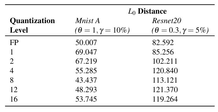
Observation 4: JSMA performs poorly in quantized net- works. The poor performance of JSMA can be explained by how JSMA creates adversarial examples. In each iteration, the JSMA algorithm seeks to find the input features that cause positive change towards the target adversarial class (Equation 15) and at the same time reduce the overall class probabilities of all other classes. When it finds these features, it adds defined amount of distortion to those features (for instance, θ = 1 and θ = 0.3 in Table 6) while also restraining total distortion to a limit (γ = 10% and γ = 5%, respectively). When networks are quantized, activation quantization makes the network insensitive to small changes in input as the small noises fail to produce any change in activations. Thus, JSMA struggles to find features that, when distorted by the defined amount, can cause misclassification.
This hypothesis was tested by randomly sampling 2,000 clean samples from MNIST and CIFAR10 datasets and creating adversarial examples using JSMA on Mnist A, Resnet20, and all their quantized versions. Average L0 distance between the adversarial samples and their corresponding benign counterparts were recorded. Three individual runs were carried out and the average L0 distance from those runs for each model are as shown in Table 7. As can be seen, on average, quantized networks required more features to be distorted than the corresponding FP model. This indicates that JSMA was struggling to find features to build adversarial examples.
Thus, although not using loss-gradients, the activation quantization causes JSMA to be less effective on quantized networks.
Table 7: Average L0 distances between the clean and adversarial samples produced using JSMA on the FP and quantized versions of Mnist A and Restnet20 models.
7.3. Summary
Based on the observations, the following statements can be made:
- MNIST models are more robust to adversarial attacks than the CIFAR10 models for some attack types. FGSM, UAP, CW attack and JSMA were found to be more effective on CIFAR10 This can be attributed to the characteristics of the data. MNIST has less variations in a single class, while CIFAR10 has larger variation of objects; thus the classifica- tion problem is simpler in case of MNIST as compared to CIFAR10. This is also reflected by the MNIST models being able to achieve very high test accuracies while the test accura- cies of the CIFAR10 models are comparatively low (Tables 2 and 3). Further, high dimensionality of CIFAR10 also causes it to have less adversarial robustness.
- Quantized networks show resistance against both gradient- based and gradient-free attacks. Activation clipping causes quantized networks to filter small noises at the input which makes the network more resilient to This was already known for attacks like FGSM and UAP from the findings in [22] and [34], respectively. This study further demonstrates that this also applies for attacks like JSMA that do not use loss gradients, for search-based attacks like the Boundary Attack, and also for the CW attack that uses logits and a more powerful objective function. Although the Boundary Attack and CW attack depicted very high effectiveness, even on quantized networks, the adversarial samples were found to be more distorted, with the Boundary Attack sometimes pro- ducing non-recognizable samples. This can be considered as a form of resilience against the attacks as the samples become more detectable and harder to create. Thus, although limited, quantization seems to provide some resistance against direct adversarial attacks.
8. Discussion
- Attacks like FGSM and UAP, which rely on loss gradients at the output layer to generate adversarial examples, tend to be less effective against quantized networks due to gradient masking [22, 34]. Interestingly, as noted in [22], CW attack demonstrated higher effectiveness in quantized networks, some extent. Furthermore, the effectiveness of some attack algorithms also depends on the characteristics of the data itself. Models trained on natural datasets like CIFAR10 seem to be more vulnerable to some attacks than those trained on datasets like MNIST. Similar observation was made in [34] for UAP attacks on SVHN and CIFAR10 datasets. We consider five different attack algorithms. FGSM is a single-step attack that uses loss gradients to create adversarial examples, whereas JSMA iteratively distorts selected pixels without relying on loss gradient information. UAP, on the other hand, focuses on finding a universal perturbation that can generalize across multiple images, rather than crafting unique adversarial samples for each one. CW attack, in contrast, performs gradient descent towards misclassification. The Boundary Attack is a gradient-free method that generates adversarial samples without requiring access to the model’s parameters or training data. Thus, the algorithms are conceptually diverse, allowing the analysis to incorporate a broader range of attack strategies and provide a more comprehensive view on adversarial robustness.
- Reproducibility is a significant challenge in Use of a single tool with well-documented functionality makes it easier for other researchers to reproduce and validate experiments. To facilitate this, we open-source our experimentation tool, ANNT. The consistent interface provided by ANNT for various tasks means that it is easier to standardize experiments and switch between different configurations. Researchers can easily share logs and configurations to replicate experiments. The resources used in the experiments in this paper, including trained models, adversarial images, and the experiment results in the form of logfiles (including those from [1]) are available at https://mega.nz/fm/public-links/ql8CwJxb. Thus, the data, along with ANNT is sufficient to replicate the experimental results.
9. Conclusion
In this work, we analyze the adversarial robustness of DNNs under direct attacks. Within this premise, we evaluate multiple attack methods on models trained on CIFAR10 and MNIST datasets and quantized to different bitwidths. Our findings, along with those from [1] indicate that quantization provides some protection against both direct and transfer-based attacks.
We also present ANNT, a tool designed to facilitate the validation of our results and support further research in this area.
- A. Shrestha, J. Großmann, “Properties that allow or prohibit transferability of adversarial attacks among quantized networks,” in Proceedings of the 5th ACM/IEEE International Conference on Automation of Software Test (AST 2024), AST ’24, 99–109, Association for Computing Machinery, New York, NY, USA, 2024, doi:10.1145/3644032.3644453.
- C. Szegedy, W. Zaremba, I. Sutskever, J. Bruna, D. Erhan, I. Goodfellow, R. Fergus, “Intriguing properties of neural networks,” CoRR, abs/1312.6199, 2014, doi:10.48550/arXiv.1312.6199.
- S.-M. Moosavi-Dezfooli, A. Fawzi, O. Fawzi, P. Frossard, “Universal adversarial perturbations,” in Proceedings of the IEEE conference on computer vision and pattern recognition, 1765–1773, 2017, doi:10.48550/arXiv.1610.08401.
- I. J. Goodfellow, J. Shlens, C. Szegedy, “Explaining and Harnessing Adversarial Examples,” arXiv preprint arXiv:1412.6572, 2015, doi:10.48550/arXiv.1412.6572.
- M. Yasmin, M. Sharif, S. Mohsin, “Neural Networks in Medical Imaging Applications: A Survey,” World Applied Sciences Journal, 22, 12, 2013.
- J. Grossmann, N. Grube, S. Kharma, D. Knoblauch, R. Krajewski, M. Kucheiko, H.-W.Wiesbrock, “Test and Training Data Generation for Object Recognition in the Railway Domain,” in P. Masci, C. Bernardeschi, P. Graziani, M. Koddenbrock, M. Palmieri, editors, Software Engineering and Formal Methods. SEFM 2022 Collocated Workshops, 5–16, Springer International Publishing, Cham, 2023, doi:10.1007/978-3-031-26236-4 1.
- E. C. Pinto Neto, D. M. Baum, J. R. d. Almeida, J. B. Camargo, P. S. Cugnasca, “Deep Learning in Air Traffic Management (ATM): A Survey on Applications, Opportunities, and Open Challenges,” Aerospace, 10(4), 2023, doi:10.3390/aerospace10040358.
- J. C.-W. Lin, G. Srivastava, Y.-D. Zhang, “Special Issue Editorial: Advances in Computational Intelligence for Perception and Decision- Making for Autonomous Systems,” ISA Transactions, 132, 1–4, 2023, doi:10.1016/j.isatra.2023.01.031.
- Y. Ijiri, M. Sakuragi, Shihong Lao, “Security Management for Mobile Devices by Face Recognition,” in 7th International Conference on Mobile Data Management (MDM’06), 49–49, IEEE, 2006, doi:10.1109/MDM.2006.138.
- A. I. Awad, A. Babu, E. Barka, K. Shuaib, “AI-powered biometrics for Internet of Things security: A review and future vision,” Journal of Information Security and Applications, 82, 103748, 2024, doi:https://doi.org/10.1016/j.jisa.2024.103748.
- H. Cui, Z. Chen, Y. Xi, H. Chen, J. Hao, “IoT Data Management and Lineage Traceability: A Blockchain-based Solution,” in 2019 IEEE/CIC International Conference on Communications Workshops in China (ICCC Workshops), 239– 244, IEEE, 2019, doi:10.1109/ICCChinaW.2019.8849969.
- N. M. Gonzalez, W. A. Goya, R. de Fatima Pereira, K. Langona, E. A. Silva, T. C. Melo de Brito Carvalho, C. C. Miers, J.-E. Mangs, A. Sefidcon, “Fog computing: Data analytics and cloud distributed processing on the network edges,” in 2016 35th International Conference of the Chilean Computer Science Society (SCCC), 1–9, IEEE, 2016, doi:10.1109/SCCC.2016.7836028.
- A. Krizhevsky, I. Sutskever, G. E. Hinton, “ImageNet Classification with deep convolutional neural networks,” Communications of the ACM, 60(6), 84–90, 2017, doi:10.1145/3065386.
- K. Simonyan, A. Zisserman, “Very Deep Convolutional Networks for Large-Scale Image Recognition,” CoRR, abs/1409.1556, 2014, doi:10.48550/arXiv.1409.1556.
- K. He, X. Zhang, S. Ren, J. Sun, “Deep Residual Learning for Image Recognition,” in 2016 IEEE Conference on Computer Vision and Pattern Recognition (CVPR), 770–778, IEEE, 2016, doi:10.1109/CVPR.2016.90.
- Y. Huang, H. Hu, C. Chen, “Robustness of on-Device Models: Adversarial Attack to Deep Learning Models on Android Apps,” in 2021 IEEE/ACM 43rd International Conference on Software Engineering: Software Engineering in Practice (ICSE-SEIP), 101–110, IEEE, 2021, doi:10.1109/ICSESEIP52600.2021.00019.
- S. Han, J. Pool, J. Tran, W. J. Dally, “Learning both Weights and Connections for Efficient Neural Networks,” Advances in neural information processing systems, 28, 2015, doi:10.48550/arXiv.1506.02626.
- R. Krishnamoorthi, “Quantizing deep convolutional networks for efficient inference: A whitepaper,” CoRR, abs/1806.08342, 2018,
doi:10.48550/arXiv.1806.08342. - A. G. Howard, M. Zhu, B. Chen, D. Kalenichenko, W. Wang, T. Weyand, M. Andreetto, H. Adam, “MobileNets: Efficient Convolutional Neural
Networks for Mobile Vision Applications,” CoRR, abs/1704.04861, 2017, doi:10.48550/arXiv.1704.04861. - Y. Guo, “A Survey on Methods and Theories of Quantized Neural Networks,” CoRR, abs/1808.04752, 2018, doi:10.48550/arXiv.1808.04752.
- Y. Zhao, I. Shumailov, R. Mullins, R. Anderson, “To compress or not to compress: Understanding the Interactions between Adversarial Attacks and Neural Network Compression,” Proceedings of Machine Learning and Systems, 1, 230–240, 2020, doi:10.48550/arXiv.1810.00208.
- R. Bernhard, P.-A. Moellic, J.-M. Dutertre, “Impact of Low-Bitwidth Quantization on the Adversarial Robustness for Embedded Neural Networks,” in 2019 International Conference on Cyberworlds (CW), 308–315, IEEE, 2019, doi:10.1109/CW.2019.00057.
- F. Tram`er, N. Papernot, I. Goodfellow, D. Boneh, P. McDaniel, “The Space of Transferable Adversarial Examples,” arXiv preprint arXiv:1704.03453, 2017, doi:10.48550/arXiv.1704.03453.
- L. Wu, Z. Zhu, C. Tai, W. E, “Understanding and Enhancing the Transferability of Adversarial Examples,” arXiv preprint arXiv:1802.09707, 2018, doi:10.48550/arXiv.1802.09707.
- A. Kurakin, I. Goodfellow, S. Bengio, “Adversarial examples in the physical world,” CoRR, abs/1607.02533, 2017, doi:10.48550/arXiv.1607.02533.
- W. Brendel, J. Rauber, M. Bethge, “Decision-Based Adversarial Attacks: Reliable Attacks Against Black-Box Machine Learning Models,” arXiv preprint arXiv:1712.04248, 2018, doi:10.48550/arXiv.1712.04248.
- N. Carlini, D. Wagner, “Towards Evaluating the Robustness of Neural Networks,” in 2017 IEEE Symposium on Security and Privacy (SP), 39–57, IEEE, 2017, doi:10.1109/SP.2017.49.
- X. Huang, D. Kroening, W. Ruan, J. Sharp, Y. Sun, E. Thamo, M. Wu, X. Yi, “A Survey of Safety and Trustworthiness of Deep Neural Networks: Verification, Testing, Adversarial Attack and Defence, and Interpretability,” Computer Science Review, 37, 100270, 2020, doi:10.48550/arXiv.1812.08342.
- N. Papernot, P. McDaniel, S. Jha, M. Fredrikson, Z. B. Celik, A. Swami, “The Limitations of Deep Learning in Adversarial Settings,” CoRR, abs/1511.07528, 2015, doi:10.48550/arXiv.1511.07528.
- A. Demontis, M. Melis, M. Pintor, M. Jagielski, B. Biggio, A. Oprea, C. Nita- Rotaru, F. Roli, “Why Do Adversarial Attacks Transfer? Explaining Transferability of Evasion and Poisoning Attacks,” in 28th USENIX security symposium (USENIX security 19), 19, 2019, doi:10.48550/arXiv.1809.02861.
- A. Krizhevsky, “Learning Multiple Layers of Features from Tiny Images,” 60, 2009.
- Y. Lecun, L. Bottou, Y. Bengio, P. Haffner, “Gradient-based learning applied to document recognition,” Proceedings of the IEEE, 86(11), 2278–2324, 1998, doi:10.1109/5.726791, conference Name: Proceedings of the IEEE.
- S.-M. Moosavi-Dezfooli, A. Fawzi, P. Frossard, “DeepFool: a simple and accurate method to fool deep neural networks,” in Proceedings of the IEEE conference on computer vision and pattern recognition, 2574–2582, 2016, doi:10.48550/arXiv.1511.04599.
- A. G. Matachana, K. T. Co, L. Mu˜noz-Gonz´alez, D. Martinez, E. C. Lupu, “Robustness and Transferability of Universal Attacks on Compressed Models,” CoRR, abs/2012.06024, 2020, doi:10.48550/arXiv.2012.06024.
- A. Madry, A. Makelov, L. Schmidt, D. Tsipras, A. Vladu, “Towards Deep Learning Models Resistant to Adversarial Attacks,” arXiv preprint arXiv:1706.06083, 2019, doi:10.48550/arXiv.1706.06083.
- N. Papernot, P. McDaniel, X. Wu, S. Jha, A. Swami, “Distillation as a Defense to Adversarial Perturbations against Deep Neural Networks,” in
2016 IEEE symposium on security and privacy (SP), 582–597, IEEE, 2016, doi:10.48550/arXiv.1511.04508. - S. Zhou, Y. Wu, Z. Ni, X. Zhou, H. Wen, Y. Zou, “DoReFa-Net: Training Low Bitwidth Convolutional Neural Networks with Low Bitwidth Gradients,” CoRR, abs/1606.06160, 2018, doi:10.48550/arXiv.1606.06160.
- Y. Bengio, N. L´eonard, A. Courville, “Estimating or Propagating Gradients Through Stochastic Neurons for Conditional Computation,” CoRR, abs/1308.3432, 2013, doi:10.48550/arXiv.1308.3432.
- M. Rastegari, V. Ordonez, J. Redmon, A. Farhadi, “XNOR-Net: ImageNet Classification Using Binary Convolutional Neural Networks,” 9908, 525–542, 2016, doi:10.1007/978-3-319-46493-0 32, series Title: Lecture Notes in Computer Science.
- M. Courbariaux, Y. Bengio, J.-P. David, “BinaryConnect: Training Deep Neural Networks with binary weights during propagations,” Advances in neural information processing systems, 28, 9, 2015, doi:10.48550/arXiv.1511.00363.
- TensorFlow Lite, “TensorFlow Lite | ML for Mobile and Edge Devices,” 2021.
- Y. Zhao, X. Gao, R. Mullins, C. Xu, “Mayo: A Framework for Auto-generating Hardware Friendly Deep Neural Networks,” in Proceedings of the 2nd International Workshop on Embedded and Mobile Deep Learning, 25–30, ACM, 2018, doi:10.1145/3212725.3212726.
- M. Jaderberg, A. Vedaldi, A. Zisserman, “Speeding up Convolutional Neural Networks with Low Rank Expansions,” CoRR, abs/1405.3866, 2014, doi:10.48550/arXiv.1405.3866.
- A. Ilyas, S. Santurkar, D. Tsipras, L. Engstrom, B. Tran, A. Madry, “Adversarial Examples Are Not Bugs, They Are Features,” Advances in neural information processing systems, 32, 2019, doi:10.48550/arXiv.1905.02175.
- Y. Liu, X. Chen, C. Liu, D. Song, “Delving into Transferable Adversarial Examples and Black-box Attacks,” CoRR, abs/1611.02770, 2017,
doi:10.48550/arXiv.1611.02770. - C. Szegedy, Wei Liu, Yangqing Jia, P. Sermanet, S. Reed, D. Anguelov, D. Erhan, V. Vanhoucke, A. Rabinovich, “Going deeper with convolutions,” in 2015 IEEE Conference on Computer Vision and Pattern Recognition (CVPR), 1–9, IEEE, 2015, doi:10.1109/CVPR.2015.7298594.
- K. Duncan, E. Komendantskaya, R. Stewart, M. Lones, “Relative Robustness of Quantized Neural Networks Against Adversarial Attacks,” in 2020 International Joint Conference on Neural Networks (IJCNN), 1–8, IEEE, 2020, doi:10.1109/IJCNN48605.2020.9207596.
- X. Huang, M. Kwiatkowska, S. Wang, M. Wu, “Safety Verification of Deep Neural Networks,” 10426, 3–29, 2017, doi:10.1007/978-3-319-63387-9 1, series Title: Lecture Notes in Computer Science.
- J. Rauber, W. Brendel, M. Bethge, “Foolbox: A Python toolbox to benchmark the robustness of machine learning models,” CoRR, abs/1707.04131, 2018, doi:10.48550/arXiv.1707.04131.
- N. Papernot, F. Faghri, N. Carlini, I. Goodfellow, R. Feinman, A. Kurakin,C. Xie, Y. Sharma, T. Brown, A. Roy, A. Matyasko, V. Behzadan, K. Hambardzumyan, Z. Zhang, Y.-L. Juang, Z. Li, R. Sheatsley, A. Garg, J. Uesato, W. Gierke, Y. Dong, D. Berthelot, P. Hendricks, J. Rauber, R. Long, P. Mc- Daniel, “Technical Report on the CleverHans v2.1.0 Adversarial Examples Library,” CoRR, abs/1610.00768, 2018, doi:10.48550/arXiv.1610.00768.
- M.-I. Nicolae, M. Sinn, M. N. Tran, B. Buesser, A. Rawat, M. Wistuba, V. Zantedeschi, N. Baracaldo, B. Chen, H. Ludwig, I. M. Molloy, B. Edwards, “Adversarial Robustness Toolbox v1.0.0,” CoRR, abs/1707.04131, 2019, doi:10.48550/arXiv.1807.01069.
- M. Courbariaux, I. Hubara, D. Soudry, R. El-Yaniv, Y. Bengio, “Binarized Neural Networks: Training Deep Neural Networks with Weights and Activations Constrained to +1 or -1,” CoRR, abs/1602.02830, 2016, doi:10.48550/arXiv.1602.02830.
- J. Uesato, B. O’Donoghue, A. v. d. Oord, P. Kohli, “Adversarial Risk and the Dangers of Evaluating Against Weak Attacks,” in International conference on machine learning, 5025–5034, PMLR, 2018, doi:10.48550/arXiv.1802.05666.
- P.-Y. Chen, H. Zhang, Y. Sharma, J. Yi, C.-J. Hsieh, “ZOO: Zeroth Order Optimization based Black-box Attacks to Deep Neural Networks without Training Substitute Models,” 15–26, 2017, doi:10.1145/3128572.3140448.
- Y. Li, X. Dong, W. Wang, “Additive Powers-of-Two Quantization: An Efficient Non-uniform Discretization for Neural Networks,” CoRR, abs/1909.13144, 2020, doi:10.48550/arXiv.1909.13144.
- Y. Netzer, T. Wang, A. Coates, A. Bissacco, B. Wu, A. Y. Ng, “Reading Digits in Natural Images with Unsupervised Feature Learning,” in NIPS Workshop on Deep Learning and Unsupervised Feature Learning 2011, 9, 2011.
- A. Shrestha, J. Großmann, “Adversarial Neural Network Toolkit,” https: //github.com/Abhishek2271/AdversarialNeuralNetworkToolkit,
2024. - M. Abadi, P. Barham, J. Chen, Z. Chen, A. Davis, J. Dean, M. Devin, S. Ghemawat, G. Irving, M. Isard, M. Kudlur, J. Levenberg, R. Monga, S. Moore, D. G. Murray, B. Steiner, P. Tucker, V. Vasudevan, P. Warden, M. Wicke, Y. Yu, X. Zheng, “TensorFlow: A system for large-scale machine learning,” OSDI’16, 21, USENIX Association, 2016, doi:10.5555/3026877.3026899.
- Y. Wu, et al., “Tensorpack,” https://github.com/tensorpack/, 2016.