Treadmill and Vision System for Human Gait Acquisition and Analysis

Adv. Sci. Technol. Eng. Syst. J. 2(3), 796–804 (2017);
 DOI: 10.25046/aj0203100
This paper presents a developed low cost system for human gait analysis. Two web cameras placed in opposite sides of a treadmill are used to acquire images of a person walking at different speeds on a treadmill, carrying a set of passive marks located at strategic places of its body. The treadmill also has passive marks with the color chosen to contrast with the ambient dominant color. The body joint angle trajectories and 3D crossed angles are obtained by image processing of the two opposite side videos. The maximum absolute error for the different joint angles acquired by the system was found to be between 0.4 to 3.5 degrees. With this low cost measurement system the analysis and reconstruction of the human gait can be done with relatively good accuracy, becoming a good alternative to more expensive systems to be used in human gait characterization.
1. Introduction
This paper is an extension of the work originally presented in 2016 IEEE International Conference on Industrial Engineering and Engineering Management (IEEM2016) [1]. The study of the human gait has been done in medical science [2-5], psychology [6, 7], and biomechanics [8-15] for more than five decades. Recently it has generated much interest in fields like robotics [16], biometrics [17] and computer animation [18]. In computer vision, recognizing humans by theirs gaits has recently been investigated [19]. The human gait is a pattern of human locomotion and can be described by kinetic or kinematics characteristics [20]. Gait signatures are the most effective and well defined representation methods for kinematic gait analysis. Gait signatures can be extracted from motion information of human gaits and have been used in computer graphics, clinical applications, and human identification [21-23].
Furthermore, gait data can be used to assess pathologies in a variety of ways. For example, stride parameters such as walking speed, step length and cadence provide an overall picture of gait quality.
Given the growing need for such analysis equipment, this paper presents a low cost system developed to characterize human gaits as an alternative to much more expensive solutions [24, 25], taking the advantage of requiring much less space for its installation (about 5 times less).
The organization of this paper is as follows: Section 2 describes the developed acquisition system and its setup. The static and dynamic performance tests are described in Section 3. The results of repeatability tests are presented in Section 4 and the conclusions in Section 5.
2. Acquisition System
The developed acquisition system is based on computer vision and tracks passive marks (circles with 4 cm of diameter) of a color chosen to contrast with the surround colors.
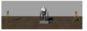
The system is mainly composed by one treadmill and two web cameras, one located on the right, and another on the left side of the treadmill, see Figure 1. Each one covers one side of the walking person.
The web cameras used have the following characteristics: CMOS 640×480 (VGA) sensor, maximum of 30 frames per second, USB 2.0 interface.
The cameras are placed at a height of 1.15 m and at a distance of 2.35 m from the treadmill. Each camera is aligned and centred to the treadmill and to the opposite camera.
After laying out the system components, the following procedures need to be followed to extract human joint angles trajectories:
A – Calibrate and align both cameras;
B – Place detection marks on the person;
C – Calibrate both sides of the pelvis;
D – Synchronize both side videos;
E – Process video frames, correct the depth of the marks, and extract joint angles.
A. Cameras Calibration and Alignment
Next it is described the cameras calibration and alignment procedures.
A.1. Cameras Calibration
When using low cost video cameras, image distortions must be considered and it is mandatory to calibrate the cameras using standard calibration procedures.
Image distortions are constant and with a calibration and remapping they can be corrected [26]. Next, it is explained the basic topics of camera calibration: radial and tangential distortion, and the perspective transformation model.
A.1.1. Radial Distortion
The radial distortion is corrected using: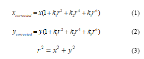
where k1, k2, and k3 are the radial distortion coefficients. Therefore, for an old pixel point at (x, y) coordinates in the input image, its position on the corrected output image will be (xcorrected, ycorrected). The presence of the radial distortion manifests in the form of the “barrel” or “fish-eye” effect.
A.1.2. Tangential Distortion
Tangential distortion occurs because the camera lenses are not perfectly parallel to the imaging plane. It is corrected by: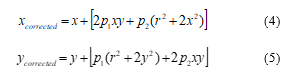
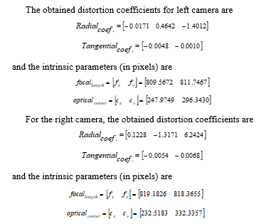
where p1 and p2 are the tangential distortion coefficients. All the five distortion parameters were calculated using the Matlab camera calibrator app.
A.1.3. Perspective Transformation Model
For the units conversion the following formula (in homogeneous coordinate system) is used: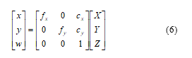
where the intrinsic camera parameters fx and fy are the camera focal lengths and (cx, cy) is the optical center expressed in pixels coordinates.
The process of determining all these nine parameters is the calibration. Calculation of these parameters is done through basic geometrical equations, and it depends on the chosen calibrating object, which was a classical black-white chessboard.
A.1.4. Camera Calibration Parameters Calculation
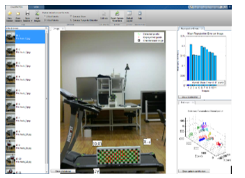
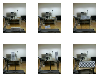
To do the calibration was used the Matlab camera calibrator app (Figure 2). The first step is to input images of a checkerboard calibration pattern. For accurate results it is recommended to use between 10 and 20 calibrating images, from each camera, and, in this case, 11 images were used (Figure 3). The checkerboard was used as calibrating object because its regular pattern make it easier to be detected automatically.
After inputting the checkerboard square size, the app will detect the checkerboard in all calibrating images. Then it is possible to inspect the results. This is helpful to find incorrect detections, and remove bad images for calibration.
After this, the calibration parameters can be calculated and if necessary images with biggest errors can be rejected and substituted by another ones to try to minimize the overall mean error.
A.2. Alignment of Cameras
Since there are two cameras and a treadmill between them, it is required to align each system component with each other to guarantee a good performance [27]. For that, it was developed a software module that measures the distance, in pixels, between six reference marks on the treadmill, and those marks viewed by the camera. Since the focal distance of the cameras and the distances between the treadmill and each camera are known, the location where the six marks should appear in the image can be calculated.
Now, it is necessary to do a manual fine alignment of the cameras in order to overlap each calculated mark position with its respective detected position in the image. Then, it is calculated the larger distance between these marks, and the goal is to ensure that the maximum distance is less than four pixels.
A. Placing Detection Marks on the Person
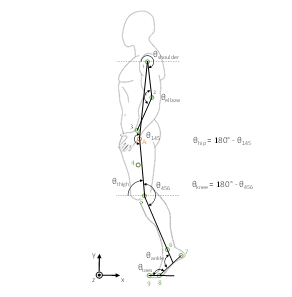
After the alignment of both cameras, it is necessary to attach 10 marks on each side of the walking person. Marks 1, 2, 3, A, 5, 6 and 8 correspond to joints in the human body: shoulder, elbow, wrist, pelvis, knee, ankle and finally finger toes, see Error! Reference source not found..
C. Pelvis Calibration
Initially, the walking person must carry twenty marks (ten on each side) placed on him, Figure 5, but after the “pelvis calibration” procedure, the pelvis marks (A in Figure 4) are removed, and the pelvis joint marks will be inferred by the extra marks placed on the upper legs (mark 4 in Figure 4).
Considering the marks do not move during data acquisition, marks 4 can be removed and their positions inferred from the positions of the other two marks. This procedure is necessary because the arm and hand occlude the pelvis marks (marks A) during gait data acquisition. Figure 5 shows the software module window for the pelvis calibration.
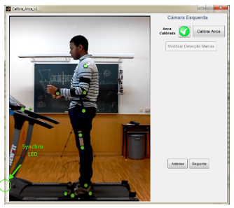
D. 3D Construction and Synchronization
To obtain 3D human gait data, it is required to cross synchronized both side’s images [28]. To synchronize cameras, there is a white synchronization LED that blinks and that is visible by both cameras (Figure 5). The video acquisition starts first, and then the synchronization LED starts blinking. The synchronization procedure is automatic and is done when processing the acquired videos, and is necessary because cameras do not start exactly at the same time and the image acquisition rate is not exactly the same for both cameras and has fluctuations.
So, it is necessary to detect on both side videos when the synchronization LED turns ON and OFF, checking if the number of frames between LED ON and OFF cycles in both videos is the same. If they are not, the marks trajectories of the side with less frames are interpolated so that both side trajectories have the same number of data. When the number of frames in deficit is equal to or greater than three, the stride where this deficit occurs is considered not okay, and is discarded. This way, both side’s videos can be crossed to extract 3D gait data.
To reference both camera images in space, there are two marks in the treadmill that are visible for both cameras (Figure 7). Both side images have their reference relative to these marks. This way it is ascertained not only the sagittal angles but also transversal and frontal rotation angles of the trunk, shoulders and pelvis.
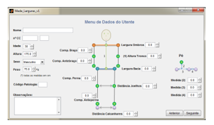
It is necessary to add depth to the person’s right and left planes, so, since the distances between all marks are measured (Figure 6), it is possible to convert those metric distances to pixels. To do this the required measures are: person height; shoulders width; arm and forearm lengths; hip width; thigh and leg lengths; distance between both ankles, and between both knees when in normal walking; great toe length; foot hinge finger to heel distance; and ankle to foot base distance. Other data are collected too, like age, gender and weight. Therefore the calculation of Body Mass Index (BMI) can be done.
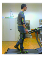
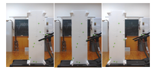
After these measurements and pelvis calibration the person walks about 6 minutes on the treadmill to be accustomed to it [29], and only after the person feels at ease with the treadmill use, the gait data acquisition can start (Figure 7).
E. Processing of Video Frames, Correcting the Depth of the Marks, and Extracting Joint Angles
After gait data acquisition, all saved data is loaded, and computed to extract the desired angle trajectories.
In this phase all frames are loaded to pass through a color segmentation process where all marks are extracted from the original videos, and the respective image coordinates are determined, [30, 31]. This segmentation is adjustable for every mark color.
The trajectories of all marks have been smoothed by using a zero lag Butterworth filter with a cut‐off frequency of 6 Hz [9, 32]. Since for speeds below 5.5 Km/h, 99.7 % of the signal power is contained in the lower seven harmonics (below 6 Hz), the use of a 6 Hz cut‐off frequency is considered to be adequate for the tests.
After being determined the coordinates of each mark for all video frames and after the noise reduction is done, each joint angle trajectory can be obtained.
Afterwards it is possible to visualize, for the entire duration of the test, the person 3D animated skeleton with all joints and links.
Stride detection makes possible stride grouping. Each stride is defined when the right foot starts going from up to down. After, the same foot stops moving forward and begins to move backward. I.e., forward to backward movement is first flagged, and after that, when upward to downward movement is detected, this instant corresponds to a new stride detection. Each stride detection ends the previous stride and starts a new one.
Figure 8 shows a window where the saved data can be viewed and analyzed.
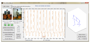
In this window it can be seen: both sides videos, the location of each detected mark (yellow circles in video frames), the angle values for all recorded person strides, a 3D animated skeleton of the person for each frame, and other options, like zoom, pan, rotate, RGB levels for mark detection, intensity threshold for synchronization LED detection, export data, etc.
At the end, all collected data can be exported and opened in another window (Figure 9), where all strides are grouped and the 17 mean joint angles profile, and their respective standard deviation (in green) are seen.
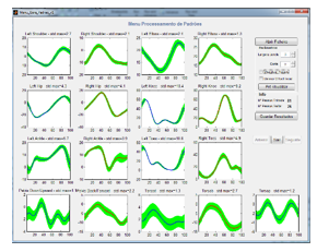
Beyond the angles referred to in Error! Reference source not found. it is also possible to extract other angles: backward/forward pelvis and trunk, downward/upward pelvis and trunk, and posterior/anterior trunk, as can be seen in Figure 10.
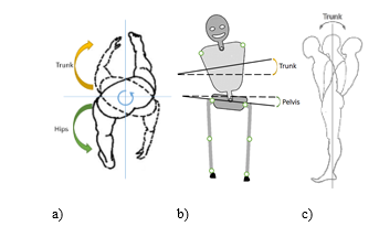
b) – Downward/Upward Trunk/Pelvis angle.
c) – Posterior/Anterior Trunk angle.
The one side marks placed on the arm and leg are in different planes (see Figure 11). Instead of considering every mark in the same plane, it was made a depth correction [33]. I.e., using the physical characteristics of the person in test (Figure 6), the difference distances between the planes were calculated. Combining the values calculated before with the physical system setup distances, the points outside of the reference plane β (like knee, ankle and every foot points) were projected to it, permitting a more accurate calculation of the angles.
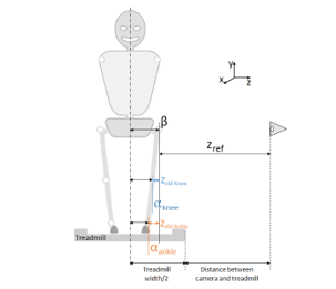
Involved variables can be viewed in Figure 12.
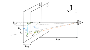
The reference plane β contains the pelvis mark point (see Figure 12).
Consider a point A with coordinates (xold,yold) on the plane α parallel to the reference plane. The new coordinates of the point A (xnew,ynew), on the reference plane β, A’, are obtained by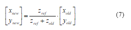
It must be mentioned that the image referential has to be at the centre of the image, and not at a corner of the image, like usually is. I.e., all of the points have to be referenced to the centre of the image.
The above procedure is executed for all points, except for pelvis point (since it is the reference point), and finally has to be done their re-reference for previous origin (original referential).
With these transformations, more accurate results are achieved.
3. Performance Tests
Static tests were performed using a static planar dummy (with known joint angles) located in three different positions on the treadmill (see Figure 13). Those angles were measured using the software and compared with the real ones to determine system static errors. Also, a dynamic test was done, where a person walked on the treadmill at different speeds. The trajectories of the joint angles were then analysed and their standard deviations were calculated to check if they were as expected, having literature trajectories as reference. A comparison between these angle profiles and the literature normal profiles was also done.
3.1 Static Tests
To determine the maximum static system error, some tests were made using a planar dummy placed at three different positions upon the treadmill: at the front, at the center, and at the rear (see Figure 13).
The planar dummy consists of two styrofoam plates with marks located as the joint positions of a human. The plates were carefully positioned in order to achieve a vertical inclination identical to that of a human (see Figure 14b). The traced and measured angles are shown in Table 1 and Table 2. These angles are defined in Figure 14.
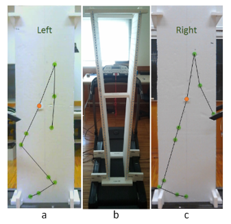
The tests were made at the three referred positions upon the treadmill to be clear that there is neither a significant error at each location, nor a relation between the location and the error.
Each test lasted 3 minutes at 30 fps, which resulted in 5400 frames. In the total of the 3 tests this corresponds to 16200 analysed frames, which are more than enough to represent accurately the precision of the system in steady state.
After analysing the results it is concluded that there was no relation between the position of the dummy on the treadmill and the error of the measurements. Table 1 and Table 2 present the maximum errors obtained in all tests.
Table 1. Measured left and right sagittal angles, and respective errors, in degrees.
| Angle
(degrees) |
Left | Right | ||||||
| Real value | Mean
meas. value |
Mean absolute error | Max. absolute error | Real value | Mean
meas. value |
Mean absolute error | Max. absolute error | |
| Shoulder | 20 | 20.4 | 0.4 | 0.7 | -20 | -19.6 | 0.4 | 0.6 |
| Elbow | -5 | -4.3 | 0.7 | 1.0 | -15 | -15.5 | 0.5 | 0.7 |
| Trunk | -20 | -21.0 | 1.0 | 1.2 | 10 | 9.7 | 0.3 | 0.5 |
| Hip | -5 | -3.7 | 1.3 | 1.8 | 5 | 6.1 | 1.1 | 1.5 |
| Knee | 65 | 64.3 | 0.7 | 1.0 | 0 | -0.3 | 0.3 | 0.6 |
| Ankle | -95 | -97.2 | 2.2 | 2.3 | -85 | -83.0 | 2.0 | 2.3 |
| Toes | -10 | -11.2 | 1.2 | 1.7 | -10 | -9.4 | 0.6 | 0.9 |
Table 2. Measured crossed angles and respective errors, in degrees.
| Angle
(degrees) |
Real value | Mean
meas. value |
Mean absolute error | Max. absolute error |
| Downward/ Upward
Trunk |
11 | 8.8 | 2.2 | 2.2 |
| Backward / Forward
Trunk |
23 | 24.1 | 1.1 | 1.2 |
| Downward / Upward
Pelvis |
9 | 7.3 | 1.6 | 1.8 |
| Backward / Forward
Pelvis |
-9 | -5.6 | 3.4 | 3.5 |
| Posterior / Anterior
Trunk |
-5 | -5.3 | 0.3 | 0.4 |
These tests show a relatively low static absolute error, with a maximum of 3.5 degrees obtained on crossed angles and 2.3 degrees on sagittal plane angles.
3.1 Dynamic Tests
A healthy person did a gait data acquisition, walking at different speeds. This person is a 30 year old male, 1.85 m tall, and weighs 87 kg.
Table 3 shows the maximum standard deviation of all angles for the different speeds of the treadmill.
Table 3. Maximum standard deviation of all angles for all dynamic tests, in degrees.
| Speed [Km/h] | 1.1 | 2.7 | 4.1 | 5.4 |
| R. Shoulder | 2.0 | 1.8 | 2.2 | 2.9 |
| L. Shoulder | 3.4 | 1.8 | 2.8 | 2.0 |
| R. Hip | 2.3 | 1.9 | 2.5 | 3.6 |
| L. Hip | 1.8 | 1.3 | 2.2 | 2.3 |
| R. Knee | 3.0 | 2.3 | 2.7 | 3.2 |
| L. Knee | 3.4 | 4.3 | 6.1 | 5.2 |
| R. Ankle | 2.0 | 1.3 | 1.6 | 2.4 |
| L. Ankle | 2.0 | 1.7 | 3.0 | 3.0 |
| Pelvis bf (1) | 1.8 | 1.4 | 1.1 | 1.7 |
| Pelvis du (2) | 0.8 | 0.7 | 0.5 | 0.8 |
| Trunk bf (3) | 2.6 | 1.9 | 1.6 | 2.1 |
| Trunk du (4) | 1.4 | 1.0 | 0.7 | 1.1 |
| Trunk pa (5) | 0.8 | 0.7 | 0.8 | 0.8 |
(1) Pelvis backward/forward, (2) Pelvis downward/upward,
(3) Trunk backward/forward, (4) Trunk downward/upward,
(5) Trunk posterior/anterior.
The maximum standard deviation of these tests is 6.1 degrees, which is similar to the value registered in [34].
Figure 15a shows the patterns of hip angles for the right side of a healthy person [35]. Figure 15b shows the measured values of the hip angle for the right side of a healthy person using the developed system.
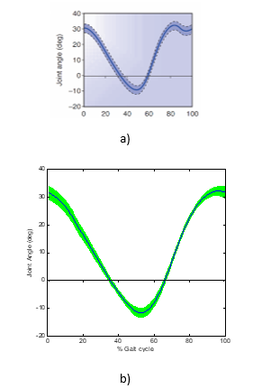
From Figure 15 it is seen that the measured values for the right hip have similar appearance to the pattern of this angle seen in the literature [35], except at the final phase of the gait cycle, where the pattern has a small nuance and our measurements do not. This nuance may be justified by the walking speed to obtain those pattern graphs, which is not mentioned in [35].
4. Repeatability Tests
Two more tests were done, where a person walked at the treadmill at different speeds and in two distinct sites. The whole system was completely installed and uninstalled in two different sites, and the same person did the gait acquisition twice, at the same speeds. The data were compared with each other, to check if both results are similar.
Figure 16 shows the mean measured values for both tests (solid lines) and their standard deviations (dashed lines). The curves obtained in both tests are similar, and their offsets are very low. The existing difference may be derived from the manual placement of each mark, which can vary, depending, for instance, on the dressing of the person.
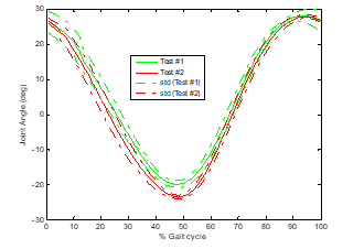
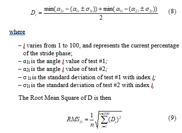
Table 4 presents the RMSD values calculated with (9).
Table 4. Root mean square of the difference, in degrees, between two similar test sets, with the same walking person, at different sites.
| Speed [km/h] | Shoulder | Hip | Knee | Ankle | ||||
| Right | Left | Right | Left | Right | Left | Right | Left | |
| 1.1 | 0.6 | 0.7 | 0.5 | 0.9 | 0.3 | 1.6 | 0.2 | 0.3 |
| 2.7 | 0.0 | 0.4 | 1.8 | 1.9 | 1.0 | 1.3 | 0.4 | 0.0 |
| 4.1 | 0.9 | 0.0 | 0.6 | 2.1 | 1.1 | 0.1 | 0.2 | 0.1 |
| 5.4 | 0.2 | 0.9 | 1.3 | 1.2 | 1.5 | 1.1 | 1.1 | 0.1 |
| Speed [km/h] | Pelvis bf (1) | Pelvis du (2) | Trunk bf (3) | Trunk du (4) | Trunk pa (5) |
| 1.1 | 2.3 | 0.9 | 0.4 | 0.4 | 0.2 |
| 2.7 | 5.0 | 1.9 | 0.3 | 0.2 | 1.2 |
| 4.1 | 3.0 | 1.9 | 0.1 | 0.2 | 0.0 |
| 5.4 | 4.1 | 1.4 | 0.5 | 0.5 | 0.9 |
(1) Pelvis backward/forward, (2) Pelvis downward/upward,
(3) Trunk backward/forward, (4) Trunk downward/upward,
(5) Trunk posterior/anterior.
It is seen that the maximum RMS difference on sagittal plane angles is 2.1 degrees for the left hip at 4.1 km/h, which is a reasonable repeatability error that is compatible with the maximum absolute error measured on static tests. For crossed angles the maximum error is 5.0 degrees at backward/forward pelvis angle at 2.7 km/h, which is a maximum error of about twice the maximum static absolute error. This is acceptable since these crossed angles are determined by crossing right side points with left side points.
With these repeatability tests it is confirmed that precision was not affected by the portability of the system.
5. Conclusions
A system for acquisition and analysis of the human gait was developed and can be used for various applications such as physiotherapy, pathology identification and rehabilitation. It presents a mean error of about two degrees, what is perfectly acceptable for human gait characterization, once the human gait presents deviations above six degrees relatively to mean values [34]. The limitation of this system is the precision on crossed angles, which, because of their side cross nature, have an error of about five degrees. However, this is not relevant for the proposed purpose of human gait characterization.
A concurrent system has a maximum error of about 0.3º, seven times lower than the presented system. However, the presented system costs about 2,500 €, is significantly cheaper than concurrent systems (20 to 40 times), presenting a high quality/price ratio.
The presented system is a simple effective solution for human gait data acquisition and characterization, with a good precision, costing much less than current systems, and having the advantage of requiring much less space for installation setup.
- Paulo A. Ferreira, João P. Ferreira, Manuel Crisóstomo, A. Paulo Coimbra, “Low Cost Vision System for Human Gait Acquisition and Characterization”, 2016 IEEE International Conference on Industrial Engineering and Engineering Management (IEEM2016), pp. 291-295, Bali, Indonésia, December 4-7, 2016.
- Michael W. Whittle, “Clinical gait analysis: A review”, USA Human Movement Science 15, 1996 Elsevier Science, 369-387.
- M. P. Murray, “Gait as a Total Pattern of Movement”, American Journal of Physical Medicine, 46(1), pp.290- 333, 1967.
- J. Perry, “Gait Analysis: Normal and Pathological Function”, Slack, 1992.
- Yuki Ishikawa, Qi An, Junki Nakagawa, Hiroyuki Oka, Tetsuro Yasui, Michio Tojima, Haruhi Inokuchi, Nobuhiko Haga, Hiroshi Yamakawa, Yusuke Tamura, Atsushi Yamashita & Hajime Asama “Gait analysis of patients with knee osteoarthritis by using elevation angle: confirmation of the planar law and analysis of angular difference in the approximate plane”, Advanced Robotics, 31:1-2, 68-79, 2017.
- G. Johansson, “Visual Perception of Biological Motion and a Model for Its Analysis”, Perception and Psychophysics, 14(2), pp.201-211, 1973.
- S. V. Stevenage, M. S. Nixon, and K. Vince, “Visual Analysis of Gait as a Cue to Identity”, Applied Cognitive Psychology, 13, pp.513-526, 1999.
- V. T. Inman, H. J. Ralston, and F. Todd, “Human Walking”, Williams & Wilkins, 1981.
- D. A. Winter, “The Biomechanics and Motor Control of Human Movement”, 4nd Eds., John Wiley & Sons, 2009.
- T. P. Andriacchi and D. E. Hurwitz, “Gait Biomechanics and the Evolution of Total Joint Replacement”, Gait and Posture, 5(3), pp.256-264, 1997.
- Ferreira, J. P., Crisóstomo, M., Coimbra, A. P., “Human Gait Acquisition and Characterization”, IEEE Transactions on Instrumentation and Measurement, Vol. 58, nº9, September 2009.
- A. Sona, R. Ricci and G. Giorgi, “A measurement approach based on micro-Doppler maps for human motion analysis and detection”, Proc. IEEE International Instrumentation and Measurement Technology Conference, pp. 354–359, May 2012.
- G. Panahandeh, N. Mohammadiha, A. Leijon, and P. Handel, “Continuous hidden Markov model for pedestrian activity classification and gait analysis”, IEEE Trans. Instrum. Meas., vol. 62, no. 5, pp. 1073–1083, May 2013.
- A. Sona, R. Ricci, “Experimental validation of an ultrasound-based measurement system for human motion detection and analysis”, in Proc. IEEE International Conference on Instrumentation and Measurement Technology (I2MTC), May 2013
- A. Balbinot, Schuck, A.,Bruxel, Y., “Measurement of transmissibility on individuals”, in Proc. IEEE International Conference on Instrumentation and Measurement Technology (I2MTC), May 2013.
- Long Y., Du Z., Dong W., Wang W. “Human Gait Trajectory Learning Using Online Gaussian Process for Assistive Lower Limb Exoskeleton”. In: Yang C., Virk G., Yang H. (eds) Wearable Sensors and Robots. Lecture Notes in Electrical Engineering, vol 399. Springer, Singapore, 2017.
- Kateřina Sulovská, Eva Fišerová, Martina Chvosteková, Milan Adámek, “Appropriateness of gait analysis for biometrics: Initial study using FDA method”, Measurement (Elsevier), Volume 105, pp 1-10, July 2017.
- Mengyuan Liu, Hong Liu, Chen Chen, “Enhanced skeleton visualization for view invariant human action recognition”, Pattern Recognition (Elsevier), Volume 68, pp 346-362, August 2017.
- M. S. Nixon, et al., “Automatic Gait Recognition”, in BIOMETRICS – Personal Identification in Networked Society, A. K. Jain, et al. Eds., pp.231-249, Kluwer, 1999.
- J. K. Aggarwal, Q. Cai, W. Liao, and B. Sabata, “Nonrigid Motion Analysis: Articulated and Elastic Motion”, Computer Vision and Image Understanding, 70(2), pp.142-156, May 1998.
- Ferreira, J. P., Crisóstomo, M., Coimbra, A. P., Carnide, D., and Marto, A., “A Human Gait Analyzer”, 2007 IEEE International Symposium on Intelligent Signal Processing-WISP’2007, Madrid, Espanha, 3-5 Outubro, 2007.
- Bux A., Angelov P., Habib Z., “Vision Based Human Activity Recognition: A Review”. In: Angelov P., Gegov A., Jayne C., Shen Q. (eds) Advances in Computational Intelligence Systems. Advances in Intelligent Systems and Computing, vol 513, Springer, 2017.
- S. K. Natarajan, X. Wang, M. Spranger and A. Gräser, “Reha@Home – a vision based markerless gait analysis system for rehabilitation at home”, 2017 13th IASTED International Conference on Biomedical Engineering (BioMed), pp. 32-41, Innsbruck, Austria, 2017.
- Vicon: Bonita. Internet, May 8, 2017, available at: http://www.vicon.com/System/Bonita.
[25] NDI Measurement Sciences: Optotrak-Certus. Internet, May 8, 2017, available at: http://www.ndigital.com/msci/products/optotrak-certus. - OpenCV: Camera calibration with OpenCV. Internet, May 8, 2017, available at: http://docs.opencv.org/doc/tutorials/calib3d/camera_calibration/camera_calibration.html.
- Miles H., Seungkyu L., Ouk C., Radu H., “Time of Flight Cameras: Principles, Methods and Applications“, Springer, 2013.
- Andrea F., Juergen G., Helmut G. Xiaofeng R., Kurt K., “Consumer Depth Cameras for Computer Vision: Research Topics and Applications “, Springer, 2013.
- Angelo Matsas, Nicholas Taylor, Helen McBurney, “Knee joint kinematics from familiarized treadmill walking can be generalized to over ground walking in young unimpaired subjects”, Elsevier, Gait and Posture 11 p46–53, 2000.
- J.J.H.López, A.L.Q.Olvera, J.L.L.Ramirez, F.J.R.Butanda, M.A.I. Manzano, D.Luz A.Ojeda, “Detecting objects using color and depth segmentation with Kinect sensor”, The 2012 Iberoamerican Conference on Electronics Engineering and Computer Science, 2012.
- Michael Van den Bergh, Luc Van Gool, “Combining RGB and ToF Cameras for Real-time 3D Hand Gesture Interaction”, IEEE Workshop on Applications of Computer Vision, 2011.
- Holden J.P, Chou G, Stanhope S.J, “Changes in Knee Joint Function Over a Wide Range of Walking Speeds”, Clinical Biomechanics Vol. 12(6): 375-382, 1997.
- P.Howard, Brian J. Rogers, “Perceiving in Depth: Stereoscopic Vision“, Vol. 2. Oxford, 2012.
- A. A. Biewener, C. T. Farley, T. J. Roberts and Marco Temaner, “Muscle mechanical advantage of human walking and running: implications for energy cost”, J Appl Physiol 97:2266-2274, 2004.
- Margareta Nordin, Victor H. Frankel, “Basic Biomechanics of the Musculoskeletal System”, 4th Edition, Wolters Kluwer, 2012.