1. Introduction

This paper is an extension of work originally presented in PlatCon-17 [1], where we show the general ideas. Significant changes are added in this extended paper to explain more about background knowledge, related work, design philosophy, and performance evaluation. Nowadays, huge volumes of data are generated on the Internet every day due to the popularity of social media and portable devices, and this opens up a new era of big data [2]. How to extract interesting information from these data has become a hot topic in science and commercial fields. Big data analytics needs the support of scalable data storage and powerful data process. Cloud computing [3], which provides distributed storage and parallel data processing on commodity computer clusters, just meets this requirement on data analysis.

Cloud computing, as defined by National Institute of Standards and Technology (NIST) [4], should be composed of five essential characteristics: broad network access, rapid elasticity, measured service, on-demand self-service, and resource pooling. Moreover, cloud computing has four basic deployment models: public cloud, private cloud, community cloud, and hybrid cloud, and has three service models: software as a service (SaaS), platform as a service (PaaS), and infrastructure as a service (IaaS).

Many large on-line services are constructed by the technique of cloud computing. These services are usually developed on business-based cloud platforms such as Amazon’s EC2, Google’s GAE, and Microsoft’s Azure. In academic research, Apache Hadoop is a popular cloud platform to test and verify research ideas. Hadoop is a Java-based and open-source software framework that supports a full set of cloud techniques: distributed file system, parallel data processing, and distributed database system.

To do parallel data processing in Hadoop, users need to write MapReduce programs [5]. These kinds of programs include two major processing codes: map and reduce to reflect a two-phase data processing flow.  The map code mainly deals with data filtering and data transforming, and the reduce code mainly deals with data aggregating. Users submit these MapReduce programs into the Hadoop system as jobs. Each job contains several map tasks and reduce tasks. The map task typically reads an input data file in the form of key-value pairs, and then generates an intermediate result file in key-value pairs as well. All values with the same key will be grouped together, and then are processed by the reduce task that usually generates aggregated values.

A Hadoop system can be built over clusters of computers that are typically named as nodes. All map and reduce tasks will be dispatched to these nodes. For parallel data processing, the input data file to a MapReduce job will be equally partitioned into several data chunks (or blocks) with a typical size of 64 MB. Each of these data chunks will be replicated and distributed into different nodes for fault tolerance. The same number of map tasks to the number of data chunks are cloned, and each copy of the map task handles one data chunk. Because there are redundant data chunks, the map task will select the closest data chunk for access efficiency. The reduce task can be cloned as well, and each copy handles the values corresponding to a certain set of keys. This MapReduce working model is outlined in Figure 1.The WordCount application that outputs the frequency of each distinct word occurred in a document file is usually used to explain the MapReduce framework. The map task will scan the input file and output the occurrence of each word in the format of (founded word, 1). Apparently, we only need to accumulate this value 1 for those outputs having the same founded word to be the word frequency. The reduce task just does this grouping and counting.

The Hadoop system can simultaneously run many map and reduce tasks from different users in a computer cluster environment. These tasks will contend system resources such as CPU, memory, and disk I/O for the completion of their jobs. Moreover, those tasks reading data chunks from far-away nodes will compete for network bandwidth. Therefore, a proper task scheduling algorithm is necessary for optimizing resource utilization and avoiding any resource starvation.

Hadoop provides three built-in scheduling modules: First-In-First-Out (FIFO) scheduler, fair scheduler, and capacity scheduler. These schedulers have their own features and have different influences on performance such as execution time and waiting time in different situations [6-10]. Fair scheduler and capacity scheduler generally perform better than FIFO scheduler. These built-in schedulers have a common drawback, which the scheduling policy is almost fixed and is not flexible to the change of working conditions. In this paper, we focus on the fair scheduler and propose some modifications to improve the scheduling throughput under the goal of resource fairness among users.

Our proposed scheduling algorithm is adaptive, because it can dynamically tune some working parameters such as the job priority and the waiting time for resource allocation. The runtime environment’s conditions such as current workload and remaining resources are considered in the determination of job running order and the amount of resources allocated to each job. A modified fair scheduler is then coded into the Hadoop system and is examined in a real testing environment. Evaluation results show that the modified fair scheduler can significantly reduce the average turnaround time of a job by over 20 percent as compared to the original fair scheduler.

The remainder of this paper is organized as follows. Section 2 briefly introduces the basic job scheduling architecture in Hadoop and the related work on scheduling algorithms. Section 3 presents and discusses the proposed five mechanisms of improving the performance of fair scheduler. Performance evaluation is conducted in Section 4. Finally, some concluding remarks are given in Section 5.

2.       Background Knowledge and Related Work

Hadoop, which is developed under the Apache projects, is an open-source software for reliable, scalable, and distributed computing. The Hadoop system is composed of two basic units: a distributed file system and a distributed data processing engine. The Hadoop distributed file system (HDFS), following the similar

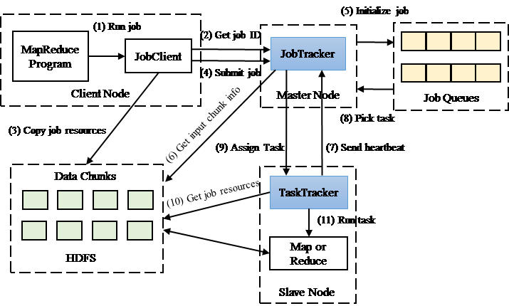
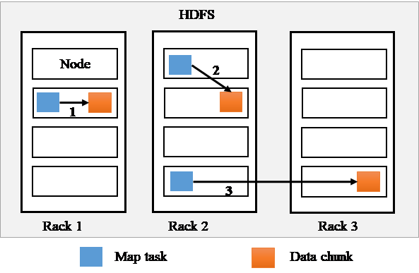
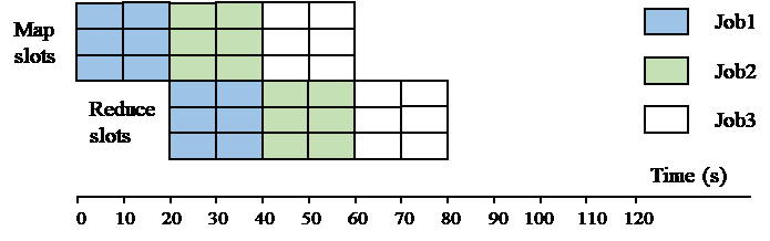
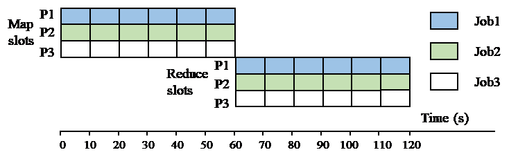
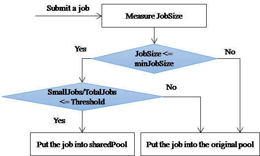
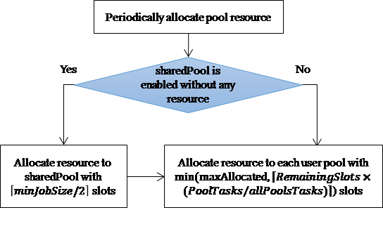
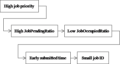
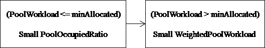
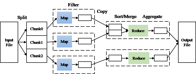Figure 1. MapReduce working model

concept of Google file system (GFS) [11], can manage distributed data storage across computer clusters built from commodity hardware. A HDFS cluster consists of a single namenode, a master server that manages the namespace and access of files, and multiple datanodes, slave servers that store data chunks and are coordinated by the master server. A file is split into several data chunks which are then stored into datanodes. The namenode will record the mapping of each data chunk to each datanode.

The distributed processing engine in Hadoop is based on the MapReduce framework. A MapReduce program contains a map procedure that performs the data filtering and sorting operations, and a reduce procedure that performs the data summarizing operations. MapReduce programs are submitted by users to Hadoop as jobs. These jobs will be executed over a set of computing nodes where one master node is selected to schedule job executions on the other slave (or worker) nodes. The management functions of system resource and job execution are included in the MapReduce module for Hadoop version 1. These functions, however, are dedicated to anther software module for Hadoop version 2: Yet Another Resource Negotiator (YARN) [12]. No matter the different versions of Hadoop, the job scheduling process is relied on a job scheduler. In this paper, we follow the framework of Hadoop version 1 to illustrate the operation of different job schedulers.

Figure 2 shows the job execution flow in Hadoop. There is a JobTracker at the master node that plays the roles of monitoring/ allocating system resources and scheduling user jobs. The JobTracker gives each submitted job a job ID as an internal identification number and puts the job into a job queue (or pool). A certain sorting policy is applied to these jobs in the queue according to some comparing factors such as job ID, job priority, and job submitted time. When a job is ready to be executed, the associated map and reduce tasks are created. The number of map tasks is determined by the number of data chunks split from an input file. The number of reduce tasks can be configured by the user but is usually one by default.

The JobTracker will manage and monitor all system resources such as CPU, memory, and disk contributed from all slave nodes. These system resources for job running are configured as resource slots in Hadoop. The resource slot used for the running of a map (or reduce) task is called a map (or reduce) slot, respectively. Due to the limited system resource, map and reduce tasks will contend these resource slots. On each slave node, a TaskTracker will manage the actual running of tasks. The TaskTracker will request a task to run from the JobTracker whenever there is a free resource slot. The TaskTracker will also periodically report the execution status and the available resource to the JobTracker by sending a heartbeat message.

Figure 2. The job execution flow in Hadoop

A map task will read an input data chuck through the HDFS. To save network bandwidth, this data retrieval should happen locally or be done from a close node. This raises the data locality issue when assigning a task to a slave node [13]. There are three levels of data localities (see Figure 3) from good to bad:

• Node-locality: The node where data are stored is the same as the node where data are processed.
• Rack-locality: The node where data are stored is different from the node where data are processed, but these two nodes are located in the same rack.
• Non-locality: The node where data are stored is different from the node where data are processed, and these two nodes are located in different racks.

Figure 3. Data locality: (1) Node-locality, (2) Rack-locality, and (3) Non-locality

The Hadoop scheduling problem can be described below: Suppose that each node is configured with some map and reduce slots for the execution of map and reduce tasks, respectively. Given a set of jobs and nodes, we need to determine the order of running jobs and the slot assignment to tasks with the objective of high data locality and high execution throughput. This problem with multi-objective optimization is proven to be NP-hard [14].

In Hadoop, there are three well-known scheduling algorithms implemented as three schedulers: FIFO scheduler, fair scheduler, and capacity scheduler, respectively. The default FIFO scheduler uses one job queue to do slot allocation. Jobs in the queue are sorted in ascending order of their submitted times. To break the tie, the job ID assigned by the JobTracker is considered. All free map and reduce slots in the system can serve the job being scheduled. In the example of Figure 4, suppose that there are three map slots and three reduce slots in the system, and each job (i.e., Job1~Job3) has three map tasks and three reduce tasks. The sequence to allocate slots to these jobs is Job1, Job2, and then Job3. For simplicity, we assume that each task uses one resource slot with the same occupation time in the figure. At first, all the map tasks of Job1 get map slots for 20 s execution time. Next, these map slots are released and re-allocated to the map tasks of Job2. Meanwhile, all the reduce tasks of Job1 get reduce slots for 20 s execution time. As can be seen, reduce tasks start executing just after the finish of all map tasks of the same job. The drawback of this scheduler is the possible long waiting time for a task to be executed when there are many jobs in the queue. This becomes unfair particularly when a user submits many jobs and the latter users need to wait.

The fair scheduler developed by Facebook equally allocates resources to job users. Each user has its own job queue (or pool), and all resource slots are fairly distributed to these user pools. Figure 5 shows the example slot allocation under the same condition with the previous example. Here three pools (P1, P2, and P3) are introduced with each pool having the resource of one map slot and one reduce slot. Each map task of these three jobs gets one map slot at the same time and runs for 20 s. The same case happens for reduce tasks. As compared to the previous example, each submitted job can start running immediately but the time to finish the job becomes longer. In a real situation, one pool without sufficient resources can borrow free (or idle) slots from another pool to increase resource utilization. To prevent resource unfairness, each pool is configured with the minimum and maximum resource capacity. Fair scheduler also supports preemptive mode by which a low-priority running job can be aborted for releasing resource to a high-priority job.

Figure 4. A scheduling example using FIFO scheduler

Figure 5. A scheduling example using fair scheduler

The capacity scheduler developed by Yahoo acts similar to fair scheduler, but uses queues instead of pools. Each queue has a defined resource capacity and is assigned to an organization or a group of users. Due to the nature of organization structure, queues can be constructed into a multi-level hierarchy. To increase running efficiency, capacity scheduler can allocate more than one resource slot to a heavy task. Moreover, several tasks can be assigned together to the same TaskTracker in batch mode to reduce the scheduling overhead. Overusing this batch mode, however, would cause load unbalancing among slave nodes. A summary table (see Table 1) is given to compare the characteristics of these three schedulers.

There are several scheduling algorithms proposed to improve the built-in schedulers. The reader is referred to [15-16] for a complete view. To increase data locality, the LATE (Longest Approximate Time to End) scheduler was proposed [17], where a delay timer is set during which a TaskTracker will wait for a suitable task that can fetch data locally. When a TaskTracker requests a task to do from the JobTracker, the JobTracker will scan the job queue to find a task with the node-locality data access level within a short time interval. If it is failed to find such a task, a task with the rack-locality data access level is then searched within a long time interval. If it is still failed, the JobTracker will randomly select one task to this TaskTracker.

The delay concept above is introduced into the naïve fair scheduler [18-19]. The setting of suitable delay time would be challenging in a dynamic changing environment. This delay time is configured as a fixed value in fair scheduler. To increase data locality, one research work implements two job queues for the FIFO scheduler [20]. Jobs having the node-locality potential are put into one queue, and jobs having the rack-locality potential are put into the other queue. Finally, these two queues are merged together and are fed into the FIFO scheduler. The process of data may have certain relationships. For example, some rare data are only processed by certain tasks. In this situation, the system can mark the locations of these rare data and assign irrelevant tasks to other locations for increasing data locality [21].

Table 1. Summary of different schedulers

Scheduler	Characteristics
FIFO Scheduler	·    Single job queue ·    Resource allocation to jobs is considered one by one. ·    Scheduling overhead is low ·    There are resource starvation problems
Fair Scheduler	·    Multiple job queues ·    Resource allocation to jobs is considered together. ·    System resources are fairly allocated to users ·    Support preemptive mode and resource borrowing
Capacity Scheduler	·    Multiple job queues ·    Resource allocation to jobs is considered together. ·    System resources are allocated to users according to a certain organization policy ·    More than one resource slot can be allocated to one task ·    Support batch mode in job scheduling

The job priority will affect the job order in a job queue. If each user can freely assign the job priority, all users tend to set their jobs to the highest level, and this does not make sense. One auto-setting mechanism is proposed in [22] by considering several factors such as the job size, the average execution time and the scheduled time of a task in a job. A high priority is usually given to a small-size or fast running job. The job size can be simply estimated by the number of tasks involved in a job [23].

In Hadoop, map slots and reduce slots are separated and cannot be interchangeably used. Dynamic borrowing between them can improve slot utilization and system throughput [24]. The map or reduce slot in Hadoop represents a computing unit and the amount of available slots in a node is configured in advance. Dynamically changing the slot number according to the real computing power in speeds of CPU and I/O can also improve system performance [25-26].

The diversity of data, jobs, and computer nodes will also affect the scheduling performance, and this is called the skew problem [27]. Different map tasks from the same job may generate different amounts of data, causing data skew. Different jobs take different execution times depending on algorithms but not job sizes, causing computational skew. Resource slots from different computer nodes have different computing powers, causing machine skew. These skews cause unbalancing workload in a distributed computer cluster. There are many research efforts on designing load balancing scheduling algorithms [28-31]. For example, jobs are classified into CPU-bound and I/O-bound types and are put into different job queues [31].

3.       Modified Fair Scheduler

Fair scheduler with the delay mechanism has good performance in general against the other schedulers in Hadoop. However, fair scheduler overemphasizes fair resource allocation to jobs and ignores the differences between jobs. These differences may even change over time when jobs are running. We hope to improve the performance of fair scheduler by considering some runtime conditions and further adjusting resource allocation to jobs. We provide some modifications to the fair scheduler by introducing the following mechanisms: job classification, pool resource allocation, resource-aware job sorting, delay time adjustment, and job priority adjustment. Their brief introductions are given in Table 2.

Table 2. The goal of each proposed mechanism

Mechanism	Goal
Job classification	Separate small-sized jobs from large-sized jobs
Pool resource allocation	Periodically reallocate resource slots to pools according to their remaining actual needs
Resource-aware job sorting	Determine the job or pool order for resource allocation based on more criteria including resource requirement and occupation
Delay time adjustment	Dynamically adjust the delay time for a suitable task with high data locality
Job priority adjustment	Dynamically adjust the job priority based on the change of its data locality level

3.1.  Job Classification

In fair scheduler, system resources are equally allocated to user pools. All jobs belonging to the same pool will contend for the limited resource. In real cases, different jobs would have different resource requirements. A large-sized job consumes more resource than a small-sized job. Based on the principle of shortest job first, we separate small-sized jobs from large-sized jobs and allocate resources to them individually.

The job size is measured by the number of map and reduce tasks in a job. In general, the number of map tasks is greater than that of reduce tasks, because most MapReduce jobs focus on data extraction from large input data sets. For simplicity, we concentrate on the map slot allocation to map tasks, so the job size is defined as the number of map tasks only. A job is recognized as a small-sized one if its job size is no greater than a threshold (minJobSize). This threshold value is not a fixed value but is updated periodically by the JobTracker (per 500 ms in our implementation) to be the currently smallest job size among all jobs in the system.

The basic concept of the proposed job classification is to direct all small-sized jobs into another system pool (called sharedPool) and all large-sized jobs into their originally belonging pools. In other words, there is a system pool shared by all users besides individual user pools. Jobs in the sharedPool are scheduled using FIFO for simplicity.

In an extreme case, if all jobs are small-sized, this job classification becomes useless. To prevent this condition, the ratio of the number of total small-sized jobs (SmallJobs) to the number of total jobs (TotalJobs) in the current system is considered. If this ratio is greater than a threshold, the sharedPool mechanism is disabled and all small-sized jobs remain in their own user pools. This threshold value is set to be the reciprocal of the average number of map slots configured in a salve node. For example, if each slave node has four map slots on average, the threshold value is 0.25. This means that we allow using sharePool when there is at most one small-sized job running on a slave node on average. Figure 6 shows the flow of job classification.

Figure 6. Job classification flow

3.2.  Pool Resource Allocation

System resources are proportionally allocated to user pools according to weighted values assigned to user pools in fair scheduler. Without the pre-knowledge of traffic shape, it is hard to set a suitable weighted value to each user pool, and this weighted value is set to be equal most of the time. However, if this weighted value can automatically reflect the current resource requirement, resource allocation can always fit real situations and becomes more efficient. Based on this concept, a dynamic pool resource allocation is proposed.

The resource allocation to pools is periodically adjusted every 500 ms in our implementation. The allocation of map slots and reduce slots to each user pool is performed separately. We first check whether the sharedPool is enabled without any allocated resource. If that is the case, a certain amount of resource slots is allocated to the sharedPool. For the efficient schedule of this small amount of small-sized jobs in the sharePool, the FIFO scheduler is applied here. We allocate a half of resource slots needed by the currently smallest job in the system to the sharedPool. That is, the number of resource slots allocated to the sharedPool is ⌈minJobSize/2⌉. This decision is for the reason that large-sized jobs should get more resource and hence we allocate limited resource to small-sized jobs. For example, if minJobSize is four in map tasks and two in reduce tasks, this sharedPool gets two map slots and one reduce slots.

The remaining free resource slots (RemainingSlots) are proportionally allocated to the other user pools according to their actual needs. The portion of total resources allocated to a user pool is based on the ratio of the number of pending tasks in a user pool (PoolTasks) to the number of total pending tasks in all user pools (allPoolsTasks). A pending task is a task that is not allocated with any resource slots and is waiting for execution. The ratio above indicates the remaining resource requirements of a user pool against the total remaining resource requirements of all jobs. Remember that only map (or reduce) tasks are considered in the counting of the number of tasks when map (or reduce) slots are allocated. To prevent one user pool with heavy workload from getting too much resource, the actual number of allocated slots cannot exceed the maximum number (maxAllocated) configured in the system. Figure 7 shows the flow of this dynamic pool resource allocation.

Figure 7. Pool resource allocation flow

3.3.  Resource-Aware Job Sorting

The order to allocate resource to jobs is based on the order of jobs. All jobs are in the same system pool for FIFO scheduler, but are in different user pools for fair scheduler. Therefore, another pool sorting is necessary besides the job sorting for fair scheduler. The job or pool order is determined based on a sorting policy applied in the FIFO comparator or the FairShare comparator in Hadoop. These two comparators, which are involved in FIFO scheduler and fair scheduler, respectively, will return the order between two target jobs or two target pools based on some reference factors. Normally, these reference factors include the job priority, job ID, and submitted time. Here, we additionally consider the remaining resource requirements and the current resource occupation of a job or a user pool to do fine-grained sorting. The principle is to allocate resource first to those jobs or pools that have occupied less resource or desire for more resource.

At first, we describe the way to determine the job order in the same pool, which can be used both in FIFO scheduler and fair scheduler. We measure the remaining resource requirements of a job by the number of pending map or reduce tasks in the job. Remember that only map tasks are counted when we consider the map slot allocation. We define the pending task ratio of a job (JobPendingRatio) in (1) as the number of pending tasks in a job to the number of total pending tasks in a pool. This ratio is high if the corresponding job has more unfinished tasks against other jobs, implying high resource requirements in the future.

JobPendingRatio = (#pending tasks in a job) ⁄ (#pending tasks in a pool)                                (1)

The current resource occupation of job is measured by the number of currently running tasks in the job. We define the occupied resource ratio of a job (JobOccupiedRatio) in (2) as the number of currently running tasks in a job to the number of totally allocated slots to a pool. If a task is assigned with at most one resource slot, the number of allocated slots is equal to the number of running tasks. A job with more occupied resource should have low precedence to contend new resource.

JobOccupiedRatio = (#running tasks in a job) ⁄ (#allocated slots to a pool)                                                                                        (2)

Our sorting policy for jobs in the same pool is designed as follows. Five comparing factors are examined in sequence if there is a tie as in Figure 8. The high order is given to the job with a high job priority (more detailed settings are discussed latter). The subsequent order is given to the job with a high JobPendingRatio and then with a low JobOccupiedRatio. To break the tie, the submitted time and the job ID are then examined.

Figure 8. Sequence to examine the job order

In fair scheduler, there are several pools and the order of these pools should be determined before jobs are scheduled. Our sorting policy for pools is also from the perspective on resource requirements. First, the number of all pending tasks for each job in a pool is accumulated as the maximal resource demand of a pool (PoolDemand) in (3). Suppose that each user pool is configured with the minimum number of resource slots (minAllocated) in advance. If PoolDemand is less than minAllocated, minAllocated would be set to be PoolDemand to reflect the actual minimum resource need. This step is for tuning the minAllocated value.

PoolDemand = ∑#pending tasks, for all jobs in a pool       (3)

Next, the number of currently running tasks for each job in a pool is accumulated as the current workload of a pool (PoolWorkload) in (4). If PoolWorkload is no greater than minAllocated, this means that the pool has sufficient resource to accommodate new tasks and hence a high pool order is given. That is, the pools are in the order of pools with sufficient resource followed by pools with insufficient resource.

PoolWorkload =∑#running tasks, for all jobs in a pool            (4)

Those pools having sufficient resource are further sorted by comparing the occupied resource ratio (PoolOccupiedRatio) of PoolWorkload to minAllocated in (5). The remaining resource is large if this ratio is low, and hence a high order is given to a pool with small PoolOccupiedRatio.

PoolOccupiedRatio = PoolWorkload ⁄ minAllocated                  (5)

Those pools having insufficient resource are further sorted by comparing the PoolWorkload and the weight of a pool that is given by the user or the system to indicate the pool priority. The ratio of these two values is computed in (6) and is denoted as WeightedPoolWorkload. A high order is given to the pool with small WeightedPoolWorkload. Here we suppose that the pool priority is high if the corresponding pool weight is large. Figure 9 shows the comparing sequence. If any tie happens, a random order is given.

WeightedPoolWorkload = PoolWorkload ⁄ (weight of a pool)        (6)

Figure 9. Sequence to examine the pool order

3.4.  Delay Time Adjustment

To increase data locality during job scheduling, JobTracker will seek first for those tasks in pools having node-locality or rack-locality levels. The setting of delay time during task scheduling is proven to be helpful on data locality. The TaskTracker will wait for a suitable task satisfying node-locality in a pool until the time out of a short delay timer. If no such task is found, the TaskTracker continues waiting for a suitable task satisfying rack-locality in a pool until the time out of a long delay timer. Otherwise, one task is randomly selected from a pool and is fed to the TaskTracker.

The fixed setting of these delay timers in the current implementation of fair scheduler is not suitable in a dynamically changing environment. A long delay timer will increase the average turnaround time of jobs, and a short delay time will decrease the average data locality level. Here, a dynamic approach is applied by setting the timer according to the recently average waiting time as follows:

NodeLocalityWaitedTime = the average waiting time of tasks satisfying node locality                                                                  (7)

RackLocalityWaitedTime = the average waiting time of tasks satisfying rack locality                                                                   (8)

In our implementation, we use two pairs of counters (TimeCount and NumberCount) to maintain each waited timer as the value of TimeCount/NumberCount. If a task is scheduled with node-locality level, the scheduled waiting time is added into TimeCount and NumberCount is increased by one. Another pair of TimeCount and NumberCount is used when a task is scheduled with rack-locality level.

3.5.  Job Priority Adjustment

In Hadoop, each job can be given with one of five priority values from high to low: VERY_HIGH, HIGH, NORMAL, LOW, and VERY_LOW. However, the job priority is not fully used and is set to a fixed value (NORMAL) without any specific specification. This priority value is one of the factors that are considered in job sorting. If this priority value can be dynamically adjusted to reflect the data locality level of a task for a job, the job with high data locality will be scheduled with high precedence. This strategy can increase overall data locality level and hence reduce the data access time.

We consider the change of the data locality level according to two recently scheduled tasks of the same job. There are nine possible changes as listed in the first column of Table 3. The job priority remains the same if there is no change on data locality. If the data locality is downgraded with one level (or two levels), the job priority is also downgraded with one level (or two levels). This job after downgrading will be sorted behind other jobs, and hence JobTracker has more opportunities to find other tasks with good data locality levels. Similarly, the job priority is upgraded with one level (or two levels) if the data locality is upgraded with one level (or two levels). If the job priority keeps in VERY_HIGH (or VERY_LOW) due to no change of data locality level, a minor adjustment to HIGH (or LOW) is applied for the balance of fairness. This prevents a job from keeping with very high or very low priority for a long period of time. The former case makes a job having high priority to seize system resource, and the latter case makes a job having the chance to starve for system resource.

Table 3. Change of job priorities

Data locality change	Original Job Priority
	VERY_HIGH	HIGH	NORMAL	LOW	VERY_LOW
NodeàNode	VERY_HIGH	HIGH	NORMAL	LOW	VERY_LOW
NodeàRack	HIGH	NORMAL	LOW	VERY_LOW	LOW
NodeàNone	NORMAL	LOW	VERY_LOW	VERY_LOW	LOW
RackàNode	HIGH	VERY_HIGH	HIGH	NORMAL	LOW
RackàRack	VERY_HIGH	HIGH	NORMAL	LOW	VERY_LOW
RackàNone	HIGH	NORMAL	LOW	VERY_LOW	LOW
NoneàNode	HIGH	NORMAL	LOW	VERY_LOW	LOW
NoneàRack	HIGH	VERY_HIGH	HIGH	NORMAL	LOW
NoneàNone	VERY_HIGH	HIGH	NOMAL	LOW	VERY_LOW

4.       Performance Evaluation

An experimental testing environment is established to evaluate the proposed fair-share-based algorithm against the original algorithm. The capacity scheduler is not examined, since it is little bit hard to configure a uniform testing environment to compare these schedulers together. Two physical computer servers are selected from two buildings on our campus. Each server is configured with four virtual machines (VMs) using the software of VMware ESXi. Each VM is installed with the operation system of CentOS 5.5 and Hadoop 1.2.1. These VMs are configured with physical IP addresses and are connected together to be one Hadoop cluster. That is, we have eight nodes in the cluster, and one node acts as both master and slave nodes and the other seven nodes act as slave nodes. Those nodes on the same physical computer are viewed as on the same rack. The hardware specification of the master node is: one dual-core CPU, 8GB memory, and 200 GB disk space. The specification of the slave node is: one dual-core CPU, 4 GB memory, and 200 GB disk space.

The replication factor of HDFS is set to three by default in Hadoop, which implies one data chunk is replicated to three nodes. However, we set the replication factor to one here and make the general node-locality level low. The reason is for the easy observation on the improvement of data locality. All the submitted jobs are based on the WordCount program which outputs the frequency of each distinct word occurred in an input document file. The job size is controlled by the size of input file. In other words, each job can contain a different number of map tasks but contain one single reduce task. The initial job priorities of all jobs are NORMAL. There are three user pools with equal weight in the system. All the submitted jobs will evenly be distributed into these pools. The minAllocated and maxAllocated values for each user pool is three and six in number of map slots, respectively. The default delay time in the original fair scheduler is 3000 ms. The above experimental settings are summarized in Table 4.

Table 4. Experimental settings

Physical server	2
Virtual machine	8
Hadoop system	1.2.1
HDFS replication	1
Default delay time	3000 ms
Job size	6~25 map tasks
User pool	3

Two sets of experiments are performed. All jobs in the first experiment have the same size, but have different sizes in the second experiment. For each experiment, two cost metrics are observed as follows:

• Average turnaround time: The average time taken between the submission of a job for execution and the completion of result output.
• Average node-locality ratio: The ratio of the number of task schedules satisfying node locality to the number of total task schedules.

4.1.  Experiment A

In this experiment, each node is configured with four map slots and one reduce slot. There are totally 32 map slots in the system. The job size (in number of map tasks) is set to be 6, 10, and 18. For each case, 5, 10, and 15 jobs are respectively examined. That is, all submitted jobs in each testing round have the same size. For this reason, the following proposed mechanisms does not contribute too much on performance improvement. First, the job classification does not work here. Second, the pool resource allocation makes no significant difference on each user pool. Therefore, we mainly observe the proposed mechanisms on resource-aware job sorting, delay time and job priority adjustments. Experimental results are listed in Table 5 and Table 6. Each gain value shown in the tables, indicating the improvement percentage, is defined as follows:

Gain = (Modified FS – Original FS) / Original FS ´ 100%       (9)

As the total number of tasks is increased, the average turnaround time is increased for both the original fair scheduler and our modified fair scheduler because of heavy workload. The modified fair scheduler can significantly reduce the average turnaround time by 21.4% to 54.5% against the original fair scheduler. This indicates that the modified fair scheduler performs proper job sorting and decreases unnecessary waiting delays. These make the utilization of resource slots high. In general, more reduction gains are achieved if the job size is getting large under the same number of jobs. This shows that the modified fair scheduler makes efficient schedule on many map tasks. The original fair scheduler will suffer from serious resource contentions under heavy workload and the lack of flexible scheduling makes the performance worse.

Table 5. Comparison of average turnaround time for jobs of same size

Job size	Number of jobs	Original FS	Modified FS	Gain (%)
6	5	289.6 s	188.2 s	-35%
	10	1083.2 s	761.3 s	-29.7%
	15	1791.7 s	1175.2 s	-34.4%
10	5	886.9 s	462.2 s	-47.8%
	10	1433.7 s	1103.3 s	-23%
	15	2008.1 s	1577.6 s	-21.4%
18	5	2212.3 s	1003 s	-54.6%
	10	3845 s	1894.1 s	-50.7%
	15	5681.4 s	2988.7 s	-47.3%

Table 6. Comparison of average node-locality ratio for jobs of same size

Job size	Number of jobs	Original FS	Modified FS	Gain (%)
6	5	0.09	0.13	+44.4%
	10	0.22	0.23	+4.5%
	15	0.28	0.28	+0%
10	5	0.29	0.32	+10.3%
	10	0.34	0.32	-5.9%
	15	0.33	0.35	+6.1%
18	5	0.21	0.25	+19%
	10	0.28	0.34	+21.4%
	15	0.3	0.36	+20%

Table 6 shows the performance comparison on data locality. First, the general node-locality ratio is low, because the replication factor is only one. Second, the node-locality ratio is improved in general by using our modified fair scheduler. Among our proposed mechanisms, only the mechanism of job priority adjustment considers the factor of data locality. Therefore, our scheduler can slightly increase the node-locality level but cannot guarantee this is always true as one counterexample in the table. Third, improvement gains become clearer when the job size is getting large. When we take a close look at the experimental result of each round, we found that data-locality levels in the original fair scheduler are variant over different testing rounds. For example, there may have several task schedules with node-locality level in the current testing round but with rack-locality level in the next testing round. However, our modified fair scheduler keeps data-locality level in a more stable state under the same input condition.

4.2.  Experiment B

In this experiment, each node is configured with two map slots and one reduce slot. There are totally 16 map slots in the system. The job sizes are mixed with five different scales: 6, 10, 16, 21, and 25. For each job size, one, two, and three jobs are respectively generated such that there are totally 5, 10, and 15 jobs in the system. All the proposed mechanisms will function in this experiment. The experimental results are listed in Table 7 and Table 8. As can be seen, the modified fair scheduler largely decreases the average turnaround time by 57% in average, and slightly increases the average node-locality ratio by 3.87% in average.

As compared to Experiment A where only three proposed mechanisms function well, improvement gains become excellent in this experiment. This means that the proposed job classification works very well and the dynamic pool resource allocation based on real resource requirement makes slot allocation more efficient.

In this experiment, we also examine the FIFO scheduler. The FIFO scheduler runs worse in the first two testing suits of Table 7, but accidently has good performance in the last testing suit. This is because that any fair-based schedulers need to set an upper bound on the number of allocated resource slots to a user pool. The performance is affected when this upper bound is reached. This setting is for allowing more users to share system resources and preventing one user to occupy all resources. The FIFO scheduler however allocates all available resources to the current user and does not consider the future resource needs for other coming users to the system. It is expected that the FIFO scheduler would perform worse when there are many users and many large-size jobs in the system.

The average node-locality ratio is close for these three schedulers as shown in Table 8. This implies that data locality is not a dominant factor on the job turnaround time. Our modified fair scheduler performs more stable and efficient than other schedulers do due to multiple considerations.

Table 7. Comparison of average turnaround time for jobs of different sizes

Job size	Number of jobs	Original FS	Modified FS	FIFO	Gain (%)
6/10/16/21/25	5	1242 s	364.6 s	513.6 s	-70.6%
	10	2343.1 s	1372.5 s	1532.2 s	-41.4%
	15	5585.3 s	2285.5 s	2131.933 s	-59.1%

Table 8. Comparison of average node-locality ratio for jobs of different sizes

Job size	Number of jobs	Original FS	Modified FS	FIFO	Gain (%)
6/10/16/21/25	5	0.25	0.26	0.27	+4%
	10	0.32	0.44	0.36	+3.8%
	15	0.32	0.44	0.36	+3.8%

5.       Conclusions

Hadoop provides parallel data processing based on the MapReduce framework. The performance of MapReduce programs is dominated by a job scheduling algorithm. Fair scheduler, which is one of the built-in schedulers in Hadoop, provides good performance in general and is widely used. However, the scheduling policy of this naïve fair scheduler is almost fixed and is not flexible to the change of working conditions. In this paper, we propose five mechanisms: job classification, pool resource allocation, resource-aware job sorting, delay time adjustment, and job priority adjustment to improve the fair scheduler by monitoring the actual resource usage and the runtime environment’s condition. The conducted experiments on a real testing platform show that the modified fair scheduler can largely reduce the average turnaround time of a job and slightly increase data locality against the naïve fair scheduler.

In the future, more types of jobs such as CPU-intensive and I/O-intensive programs will be conducted in the experiment. Also, our current work only emphasizes the slot allocation and data locality for map tasks, more enhancements for reduce tasks can be furthered considered.

Acknowledgment

The authors would like to thank the anonymous referees for their helpful suggestions. This research was partially supported by Ministry of Science and Technology of the Republic of China under Contract No. MOST 104-2221-E-259-016.

1. Y. W. Cheng and S. C. Lo, “Improving Fair Scheduling Performance on Hadoop,” in Intl. Conf. on Platform Technology and Service, Feb. 2017.
2. A. Labrinidis and H.V. Jagadish, “Challenges and opportunities with big data,” in VLDB Endowment, 5(12), 2032-2033, Aug. 2012.
3. M. Armbrust, A. Fox, R. Griffith, and A. D. Joseph et al., “A view of cloud computing,” Communications of the ACM, 53(4), 50-58, Apr. 2010.
4. The NIST Definition of Cloud Computing, Sept. 2011, http://dx.doi.org/10.6028/NIST.SP.800-145
5. J. Dean and S. Ghemawat, “MapReduce: simplified data processing on large clusters,” Communications of the ACM, 51(1), 107-113, Jan. 2008.
6. S. Liu, J. Xu, Z. Liu, and X. Liu, “Evaluating task scheduling in Hadoop-based cloud systems,” in IEEE Intl. Conf. on Big Data, 47-53, Oct. 2013.
7. A. Rasooli and D. G. Down, “A hybrid scheduling approach for scalable heterogeneous Hadoop systems,” in SC Companion: High Performance Computing, Networking Storage and Analysis, 1284-1291, Nov. 2012.
8. Y. Chen, A. Ganapathi, R. Griffith, and R. Katz, “The case for evaluating MapReduce performance using workload suites,” in IEEE Intl. Symposium on Modeling, Analysis & Simulation of Computer and Telecommunication Systems (MASCOTS) , 390-399, Jul. 2011.
9. L. Li, Z. Tang, R. Li, and L. Yang “New improvement of the Hadoop relevant data locality scheduling algorithm based on LATE,” in Intl. Conf. on Mechatronic Science, Electric Engineering and Computer (MEC), 1419-1422, Aug. 2011.
10. K. Yamazaki, R. Kawashima, S. Saito, and H. Matsuo, “Implementation and evaluation of the JobTracker initiative task scheduling on Hadoop,” in Intl. on Symposium Computing and Networking (CANDAR), 622-626, Dec. 2013.
11. S. Ghemawat, H. Gobioff, and S. T. Leung, “The Google file system,” in ACM Symposium on Operating Systems Principles (SOSP), 29-43, Oct. 2003.
12. V. K. Vavilapalli et al., “Apache Hadoop YARN: yet another resource negotiator,” in Annual Symposium on Cloud Computing, Oct. 2013.
13. J. Xie, S. Yin, X. Ruan, and Z. Ding et al., “Improving MapReduce performance through data placement in heterogeneous Hadoop clusters,” in IEEE Intl. Symposium on Parallel & Distributed Processing, Workshops and Phd Forum (IPDPSW), 1-9, Apr. 2010.
14. D. A. Heger, “Optimized resource allocation & task scheduling challenges in cloud computing environments,” dheger@dhtusa.com, 2010.
15. B. T. Rao and L. S. S. Reddy, “Survey on improved scheduling in Hadoop MapReduce in cloud environments,” Intl. Journal of Computer Applications, 34(9), 29-33, Nov. 2011.
16. N. Tiwari, S. Sarkar, U. Bellur, and M. Indrawan, “Classification framework of MapReduce scheduling algorithms,” ACM Computing Surveys, 47(3), Apr. 2015.
17. M. Zaharia, A. Konwinski, A. D. Joseph, R. Katz, and I. Stoica, “Improving MapReduce performance in heterogeneous environment, ” in USENIX Conf. on Operating Systems Design and Implementation, 29-42, Aug. 2008.
18. M. Zaharia, D. Borthakur, J.S. Sarma, and K. Elmeleegy et al., “Delay scheduling: a simple technique for achieving locality and fairness in cluster scheduling,” in Proc. European Conf. on Computer Systems, 265-278, Apr. 2010.
19. M. Zaharia, D. Borthakur, J. S. Sarma, and K. Elmeleegy et al., “Job scheduling for multi-user map reduce clusters,” ECS Department, University of California, Berkeley, Apr. 2009.
20. H. Zhao, S. Yang, Z. Chen, H. Yin, and S. Jin, “A locality-aware scheduling based on a novel scheduling model to improve system throughput of MapReduce cluster, ” in Proc. Intl. Conf. on Computer Science and Network Technology (ICCSNT), 111-115, Dec. 2012.
21. T. Y. Chen, H. W. Wei, M. F. Wei, and Y. J. Chen et al., “LaSA: A locality-aware scheduling algorithm for Hadoop-MapReduce resource assignment,” in Proc. Intl. Conf. on Collaboration Technologies and Systems (CTS), 342-346, May 2013.
22. P. Nguyen, T. Simon, M. Halem, D. Chapman, and Q. Le, “A hybrid scheduling algorithm for data intensive workloads in a MapReduce environment,” in IEEE Intl. Conf. on Utility and Cloud Computing (UCC), 161-167, Nov 2012.
23. M. Pastorelli, A. Barbuzzi, D. Carra, M. Dell’Amico, and P. Michiardi, “HFSP: size-based scheduling for Hadoop,” in IEEE Intl. Conf. on Big Data, 51-59, Oct. 2013.
24. S. Tang, B. S. Lee, and B. He, “Dynamic slot allocation technique for MapReduce clusters,” in IEEE Intl. Conf. on Cluster Computing (CLUSTER), 1-8, Sept. 2013.
25. S. Tang, B. S. Lee, and B. He, “DynamicMR: A dynamic slot allocation optimization framework for MapReduce clusters,” IEEE Trans. on Cloud Computing, 2(3), 333-347, Jul.-Sept. 2014.
26. S. Kurazumi, T. Tsumura, S. Saito, and H. Matsuo, “Dynamic processing slots scheduling for I/O intensive jobs of Hadoop MapReduce,” in Intl. Conf. on Networking and Computing (ICNC), 288-292, Dec. 2012.
27. Y. Kwon, M. Balazinska, B. Howe, and J. Rolia, “Skew-resistant parallel processing of feature-extracting scientific user-defined functions,” in ACM Symposium on Cloud computing (SoCC), Jun. 2010.
28. B. S. Kapil and S. S. Kamath, “Resource aware scheduling in Hadoop for heterogeneous workloads based on load estimation,” in Intl. Conf. on Computing, Communications and Networking Technologies (ICCCNT), 1-5, Jul. 2013.
29. Y. Le, J. Liu, F. Ergun, and D. Wang, “Online load balancing for MapReduce with skewed data input,” in IEEE INFOCOM Conf., Apr. 2014.
30. X. Xu, L. Cao, and X. Wang, “Adaptive task scheduling strategy based on dynamic workload adjustment for heterogeneous Hadoop cluster,” IEEE Systems Journal, 10(2), 471-482, Jun. 2016.
31. S. Y. Hsieh, C. T. Chen, C. H. Chen, H. C. Hsiao, and R. Buyya “Novel scheduling algorithms for efficient deployment of MapReduce applications in heterogeneous computing environments,” IEEE Trans. on Cloud Computing, http://doi.ieeecomputersociety.org/10.1109/TCC.2016.2552518

(Click to view)

(Click to view)