1          Introduction

This paper is an extension of work originally presented in the 2016 IEEE/SICE International Symposium on System Integration [1]. This previous work proposed a monocular height estimation method by chronological correction of road unevenness, which basic experiments in laboratory and asphalt correcting camera pitch variations proved the validity of the method. However, since only pitch variations were considered and experiments were conducted on asphalt in one environment, several items remained as future work. Therefore, we extended our work by the following:

• Analysis and 3 degree-of-freedom (3DOF) com-pensation of errors caused by roll, pitch and yaw variations.
• Extended experiments on asphalt with severalconditions of road and objects, permitting further analysis of external disturbances.

Cameras have been applied in many fields such as robotics and autonomous driving for localization and object recognition [2]-[7]. Even though stereo cameras can provide the depth to obstacles, their higher cost and required processing have motivated several studies to estimate depth or height with monocular cameras. Height estimation permits the robot to detect and avoid potential obstacles on the road, becoming a valuable information of the surrounding environment. Studies [8] and [9] estimate height of objects with a steady camera. While the first relies on a previous calculation of the vanishing point, the latter relies on a known object height in the scene. On the other hand, other studies focus on height estimation using a moving camera. Study [10] estimates height by computing the focus of expansion in the scene and segmenting ground and plane by sinusoidal model fitting in reciprocal-polar space. The method proposed in [11] estimates height of objects on the road by obstacle segmentation and known camera displacement from odometric measurements, refining the measurements with several frames. Although there are many promising height estimation methods, they still strongly rely on extra extraction of information from the scene or external sensors. Moreover, the presented methods assume that the ground is flat and no discussions or analyses of eventual pose variations of the camera were mentioned. In this context, we propose in this work a height estimation method that requires no previous information of the scene, nor information from

external sensors. Furthermore, even though we assume flat surface, we analyze and compensate the effects of roll, pitch and yaw variations of the camera.

The rest of this paper is organized as follows. Section 2 introduces the existing issues of monocular cameras due to depth ambiguity and roll, pitch and yaw variations. Section 3 explains the proposed monocular height estimation method and compensations of roll, pitch and yaw variations. The conducted experiments are detailed in section 4. The obtained results are discussed in section 5. Lastly, the conclusions and future work are provided in section 6.

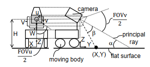Figure 1: Conversion between pixels and meters using the Flat Surface Model.

2          Issues of Monocular Cameras

In this section, two main issues of monocular cameras are introduced: A) depth ambiguity and B) effects of roll, pitch and yaw variations.

2.1         Depth Ambiguity

In order to explain this limitation, we first briefly introduce the Flat Surface Model (FSM), a technique that permits easy relation of pixels (in camera coordinates) and meters (in real world coordinates), and is commonly applied with monocular cameras [12]-[14]. Figure 1 shows a moving body, a camera and flat surface. The camera is attached to the moving body at a known height H and angle α in relation to the flat surface. The line connecting the camera center and the flat surface with angle α is called principal ray. The coordinate system of the camera is defined by pixels (u,v), with a known and fixed vertical length V and a horizontal length W. The maximum angle seen by the camera (field of view) in both u and v directions are fixed and defined as angles FOVu and FOVv. The coordinate system defined by (X,Y,Z) is fixed on the moving body. If we assume that the surface is flat, the relation between a pixel (u,v) and its real position (X,Y,Z) in meters is given by (1) to (3), where β is the angle in relation to the principal ray.

(2v − V )           FOV v β = atan(                 tan(              )) V                     2	(1)
H Y = tan(α +β)	(2)
cos(β)      (2u − W)           FOV u X = Y                                         tan(              )	(3)

                             cos(α +β)        W                     2

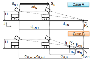Figure 2: Example of application (A) and limitation (B) when applying the Flat Surface Model.

One common application of the FSM is to estimate the camera displacement by Visual Odometry (VO) [12]-[14], which is briefly explained in “Case A” of Figure 2. First, consider the moving body and camera described in Figure 1 running on a flat surface. In an initial position S_N−₁, the camera takes a frame and shoots a point P_R on the ground, computing Y_N−₁ = d_R,N−₁. Next, consider that the moving body moves ∆d_N in direction I of a coordinate system (I,J) fixed on the ground, reaching position S_N . In this new position, it takes another frame, tracks point P_R and Y_N = d_R,N is obtained by the FSM. Using the computed information Y_N−₁ and Y_N from the two positions S_N−₁ and S_N , the real camera displacement ∆Cam_N can be correctly estimated by (4). By repeating the previous steps, the displacement of the moving body can be estimated on the following positions. Notice that we showed a simple case with only one point P_R and direction I, but many points and directions can be considered in VO.

                           ∆CamN = dR,N−1 − dR,N = ∆dN                                   (4)

The depth ambiguity can be visualized in “Case B” of Figure 2, which contains an object of height h on the ground. Let’s assume that in position S_N−₁ the camera shoots a point P_R⁰ on the top of the object, and the projection on the flat surface is point P_{P ,N}−₁, exactly on the same location as point P_R in “Case A”. Although points P_R and P_R⁰ belong to different (X,Y,Z) in the world, the FSM can’t distinguish this ambiguity and computes Y_N−1 = ^d_R,N⁰ ₋₁ = d_R,N−1. However, when the camera moves ∆d_N in direction I, it tracks point P_R⁰ and consequently, computes Y_N = d_R,N⁰ at position S_N . Finally, the displacement ∆Cam⁰_N seen by the camera becomes as (5), what shows that the real displacement ∆d_N is not correctly estimated due to the presence of the object.

∆Cam0N = dR,N0     −1 − dR,N0 ,∆dN                                (5)

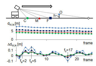Figure 3: Influences of pose variation on the Flat Surface Model.

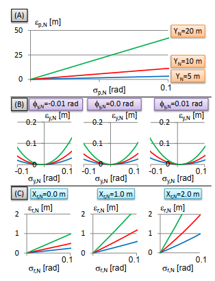Figure 4: Expected errors of the calculated distances by the FSM in function of pitch (A), yaw (B) and roll (C).

2.2         Effects of Roll, Pitch and Yaw Variations

Even though the FSM assumes that the surface is perfectly flat, in fact small unevennesses exist. Such influences are detailed in Figure 3, with a simple analysis done on a real asphalt. A camera was fixed on a moving body and moved tracking four points: i) on a static object with height h (point O), ii) on the ground far from the camera (point F), iii) on the ground close to the camera (point C) and iv) on the ground with a distance between F and C (point M). In each frame, the distances Y_N = d_W,N obtained by the FSM were computed. In order to better visualize the influences of unevennesses, the corresponding displacements ∆d_W,N = d_W,N − d_W,N−1 are also displayed in the figure. If the surface of the asphalt was really flat, then the displacements ∆d_W,N of each point C, M and F were expected to be the same in each frame. However, while this happened in frame f_a = 2 for example (suggesting that the pose of the camera was exactly the one expected by the FSM), in frames f_b = 5 and f_c = 17 the displacements were different (suggesting that the pose of the camera was different from the one expected by the FSM). Moreover, Figure 3 shows another important pattern, which points closer to the camera have smaller magnitudes of ∆d_W,N : the magnitude of ∆d_W,N calculated with C in a determined frame is smaller than the one calculated with M, which is smaller than the one calculated with F, which is smaller than the one calculated with O in the same frame. This example clearly shows the effect of unevennesses on the FSM. A further analysis according to roll, pitch and yaw variations is presented in Table 1 and Figure 4.

2.2.1        Pitch

Figure (a) of Table 1 shows the influence of pitch variations on the FSM. Consider that in a certain frame N a moving body that is shooting a point O_R on a static object on the surface has its pitch changed (represented by σ_p,N ) by an unevenness. This variation shifts height H to H_p,N and therefore the camera computes the distances by the FSM in relation to a new wrong flat surface, FS_p,N . In this wrong surface, the projection of point O_R becomes P_p,N and consequently, Y_N = d_p,N is calculated. However, the correct distance in such configuration is the one computed with G_R, the projection of O_R on the real surface on the ground, resulting in Y_N = d_R,N . The relation between the wrong (d_p,N ) and correct (d_R,N ) distances is shown by (6), (7) and (8), where l_p is the axis of rotation and γ_p,N is the angle between the camera height H and l_p. It is important to notice that the presented equations don’t explicitly contain the object height h. It happens because the computed Y_N = d_p,N itself contains this information, since it is function of O_R, P_p,N and h. We define the error caused by pitch variation σ_p,N as ε_p,N , which is the difference between the wrong estimated distance (d_p,N ) and correct one (d_R,N ), according to (9). Figure 4 (A) quantifies this error ε_p,N by adopting as example H = 1.65 m, l_p = 1.03 m, several camera pitch variations (σ_p,N ) and apparent distances to a point by the FSM (Y_N = d_p,N ). The adopted values of the constant parameters H and l_p are the same as the ones used in the experiments section for easier analysis of the obtained results. We can observe that ε_p,N increases with the increase of σ_p,N and Y_N . Even for a pitch variation of σ_p,N = 0.1 rad, the error ε_p,N can reach nearly 50 m when Y_N = 20 m, what shows that ε_p,N is very sensitive even to small σp,N .

Variation	Compensation
(a) pitch	γp = arctan(          )               (6) q Hp,N =          lp2 +H2sin(σp,N +γp)                  (7) dR,N = q Hp,N [(dp,N +lp)cos(σp,N ) −                  lp2 +H2cos(σp,N +γp)] Hp,N − (dp,N +lp)sin(σp,N ) (8) εp,N = |dR,N − dp,N |                           (9)
(b) yaw	Xy,N )      (10) d q dR,N =       Xy,N2     +dy,N2 cos(σy,N − φy,N )            (11) εy,N = |dR,N − dy,N |                         (12)
dR,N                                                                                                               unevenness (c) roll	H γr = arctan(          )               (13) q Hr,N =           lr2 +H2sin(σr,N +γr)                 (14) H dR,N = r,N − (lrr,N+Xdrr,N)sin(σr,N )                 (15) H εr,N = |dR,N − dr,N |                          (16)

Table 1: Error compensation of the calculated distances by the FSM caused by variations of roll, pitch and yaw.

2.2.2        Yaw

Figure (b) of Table 1 describes the influence of yaw variations on the FSM. Consider that in a certain frame N, a moving body that is shooting a point O_R on a static object on the surface has its yaw changed (σ_y,N ). In the former pose (pose_N⁰ ), the camera computes the distance to point G_R as Y_N = d_y,N and X_N = X_y,N . However, the correct distance in Y direction in the new pose (pose_N ) is d_R,N . Equations (10) and (11) show the relation between the wrong and correct distances, where φ_y,N is the angle in which the camera sees the object in the former pose. The error ε_y,N caused by σ_y,N is defined as (12). Figure 4 (B) shows error ε_y,N in function of yaw variation (σ_y,N ), φ_y,N and apparent distance to the point (Y_N = d_y,N ). First, when φ_y,N = 0 rad, we can observe that ε_y,N increases with the increase of Y_N and absolute value of σ_y,N . For similar conditions of Y_N and σ_y,N , when φ_y,N , 0 the errors are shifted to the left or right according to the value of φ_y,N . From this analysis we can observe that small yaw variations such as σ_y,N = 0.1 rad results in ε_y,N > 0.1 m for the adopted range of the parameters in the example, what shows that yaw variations cause smaller errors in the distances computed by the FSM comparing to the pitch variations.

2.2.3        Roll

Finally, Figure (c) of Table 1 shows the influence of roll variations on the FSM. Consider a camera tracking a point O_R on a static object of height h on the surface in a certain frame N. In the same frame, the moving body is affected by an unevenness on the flat surface, varying its roll (σ_r,N ). This variation changes height H to H_r,N and the camera computes the distances by the FSM in relation to a wrong flat surface, FS_r,N . In this wrong surface, the projection of point

O_R becomes P_r,N and Y_N = d_r,N is calculated. However, the correct distance is the one computed with G_R, the projection of O_R on the real surface on the ground, resulting in Y_N = d_R,N . The relation between the wrong (d_r,N ) and correct (d_R,N ) distances is shown by (13), (14) and (15), where l_r is the axis of rotation and γ_r,N is the angle between the camera height H and l_r. We define the error caused by roll variation σ_p,N as ε_p,N , which is the difference between wrongly estimated distance (d_r,N ) and correct one (d_R,N ), as shown in (16). Figure 4 (C) shows error ε_r,N in function of camera roll variation (σ_r,N ), X_r and apparent distance to the point (Y_N = d_r,N ). We can observe that ε_r,N increases with the increase of σ_r,N , X_r and Y_N . For roll variations of σ_r,N = 0.1 rad, ε_r,N > 2.0 m can occur for the adopted range of the parameters in the example, but those errors are still smaller than the ones caused by pitch variation.

3          Proposed Method

This section is divided into three parts: A) proposed height estimation method, B) compensation of roll, pitch and yaw variations and C) proposed algorithm.

3.1         Proposed Height Estimation

Although the FSM has the ambiguity limitation when computing VO, in fact, the difference of the obtained displacements caused by the object (∆Cam_N , ∆Cam_N⁰ ) contains useful information. First, the presence of objects in the scene influence the apparent displacements in pixels seen from the camera. Such difference in apparent displacements is explored in [12] to find irregularities in the optic flow and detect precipices. On the other hand, no further information can be extracted by existing techniques. Here, our method is based on the principle that since the FSM assumes known H and α, then we can assume that the resulting projections are also function of these dimensions. If we further observe the geometrical relations caused by the FSM and triangulation in two positions (Case B in Figure 2), we can in fact obtain geometrical relations in function of H and α, as shown in (17), (18) and

(19). From these equations and (4), we obtain (20) to (22). Several relations can be observed from the equations. First, the object causes an extra amount of apparent displacement, defined as m_N , and it is proportional to the object height h and camera height H. Second, the object height is function of the correct camera displacement ∆Cam_N and wrong apparent displacement ∆Cam_N⁰ . As afore mentioned, ∆Cam_N can be estimated by traditional VO and even though this technique will be applied, it is not the focus of this work.

                                        H                  h

	= dR,N−1   mN +nN	(17)
	H           h 0          = dR,N           nN	(18)
	dR,N0     = dR,N − mN	(19)
0		(20)
∆CamN = dR,N−1 − dR,N +mN = ∆CamN +mN

                      h(dR,N−1 − dR,N0   )      h(dR,N0 −1 − dR,N0  )

          m_N =                                   =                                          (21)

                                   H                                  H

∆Cam^N

                                   h = H(1 ⁻  ₀ )                          (22)

∆Cam_N

Roll, pitch, yaw compensation

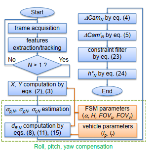Figure 5: Flowchart of the proposed height estimation method and compensations.

3.2               Compensation of Roll, Pitch and Yaw Variations

The equations displayed in Table 1 show that the compensation of the influences caused by roll, pitch and yaw are straightforward and can be easily done if σ_p,N , σ_y,N are σ_r,N are known. Thus, for each acquired frame by the camera, we compute these variations and substitute them with the constant and known parameters of the vehicle (l_p, l_r) and the FSM (α, H, FOV_u, FOV_v) in (8), (11) and (15), obtaining the compensated value d_R,N . The main steps of the proposed compensations are illustrated in the bottom part of Figure

5.

3.3         Proposed Algorithm

Figure 5 summarizes the flow of the proposed algorithm. Frames are acquired, features are extracted and tracked in two frames. Next, the corresponding values of X and Y are computed by the FSM. Roll, pitch and yaw variations (σ_p,N , σ_y,N , σ_r,N ) are estimated by VO and we compensate their influences using (8), (11) and (15), as explained in the previous section. The camera displacement (∆Cam_N ) and compensated apparent displacement of the object (∆Cam⁰_N ) are calculated by the FSM. Here, we propose to apply two filters. First, a filter based on displacement constraints to verify the applied compensations. Even though the compensations strongly rely on the estimated roll, pitch and yaw, wrong estimations on the contrary lead to high errors. The filter works according to the observed in Figure 3. If a tracked point belongs to an object above the surface, then its apparent displacement must be bigger than the camera displacement (∆Cam_N < ∆Cam⁰_N ). Therefore, we check this condition by calculating the apparent displacement of the object with (∆Cam^0c_N ) and without (∆Cam^0nc_N ) compensations. If one of them satisfies the condition, then we adopt this displacement as ∆Cam⁰_N . If both or none of them satisfies the condition, then we use the average of the two displacements to estimate the height, as show in (23). Finally, the median (h^∗_N ) of the previous estimations (h₁,h₂,…,h_N−₁,h_N ) is also applied to filter eventual noises, as (24).

∆Cam⁰_N =

            0c ∆Cam N              0nc  ∆Cam N           0nc                 0c              N +∆Cam N ∆Cam  2

if ∆Cam0cN > ∆CamN > ∆Cam0ncN if ∆Cam0cN < ∆CamN < ∆Cam0ncN otherwise (23)

                          h^∗_N = median(h₁,h₂,…,h_N−1,h_N )                   (24)

4          Experiments

The proposed method was evaluated with data from the KITTI Vision Benchmark Suite (called hereon as “KITTI”) [15] and processed with a computer Intel(R) Core(TM) i7-4600, 2.10 GHz, operating system Ubuntu (TM) 14.04, Eclipse (TM) development environment and OpenCV libraries [16]. Here, we want to verify the validity and effectiveness of the proposed height estimation and the proposed compensations of errors caused by roll, pitch and yaw variations. Thus, all estimated heights were done with two methods for later comparison: i) with roll, pitch and yaw compensation and ii) without compensation.

4.1         Applied VO

In order to estimate the camera displacement ∆Cam_N in each frame, we adopted a simple VO with rotation estimation by Nister’s 5-point algorithm [17] and translation by the FSM using features in a ground region close to the camera (details in the Appendix section), similarly to [12]. The parameters (FOV_u,FOV_v, W, V, H, etc) necessary for the experiments were adopted according to the provided by the KITTI. The camera inclination in relation to the ground was not directly provided, but we estimated that α = 1.1^o using the provided velodyne data. The feature extractor applied was FAST [18]. The features were automatically extracted when their number was bellow 1500 features. In order to evaluate the proposed monocular height estimation method, only the left images of the grayscale camera of the KITTI were used.

4.2         Evaluation Criteria

The evaluation was based on the error (ε_N ) between the ground truth (h_{GT ,N} ) and the estimated height (h^∗_N ) in each frame N, according to (25). The ground truth adopted was mainly the height provided by the velodyne, available in the KITTI. Further details can be found in the Appendix section.

                                    εN = |hGT ,N − h∗N |                             (25)

We also adopted a criterion to consider if the height estimation in a frame failed or not. For example, since we considered only objects above the ground surface, the estimated heights must be higher than 0 m (i.e., h_min = 0). Furthermore, since the FSM considers objects below the horizon line, all objects used in the experiment should have maximum height equal to the camera height (h_max = H). All estimated heights outside this maximum and minimum were considered as failure, as detailed in (26).

^_^success               h height estimation = ^

                                            ^_failure     otherwise

(26)

4.3         Results

Experiments were conducted with 10 video sequences of the KITTI, which contained many static objects (parked cars, poles, fences, houses, people, boxes, etc) in the scene. In total, height was estimated 4561 times with 436 objects. Objects with height 0 ≤ h ≤ H and distance from 4 to 31 m from the camera were used. The obtained results are summarized in Table 2, Table 3 and Figure 6.

Data	Video sequence	Valid	Valid
	(KITTI)	frames	objects
1	00	1103	85
2	05	384	35
3	07	229	18
4	08	373	29
5	09	228	23
6	13	347	43
7	15	471	32
8	16	361	35
9	18	407	32
10	19	1094	104
total	–	4997	436

Table 2: Summary of the conducted experiments.

	without	with
	comp.	comp.
comp. parameter	–	pitch, yaw, roll
average εN [m]	0.23	0.20
maximum εN [m]	1.51	1.12
number of failures	283	65

Table 3: Comparison of the obtained errors with and without the proposed compensations.

₂ N [m]                                                            ₂ _N [m]

11

00

       0      400    800   1200        0                           400

 

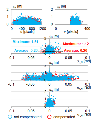Figure 6: Obtained errors of the estimated heights of all data in the experiments. The results are displayed according to pixels (u,v) and unevennesses (σ_p,N , σ_y,N , σr,N ).

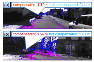Figure 7: Maximum error cases with and without compensation.

5          Discussions

Table 2 shows the 10 data and corresponding video sequence belonging to the KITTI. The number of valid frames and objects used in each data are also displayed. The estimated heights of all objects chosen within this data are presented in relation to the pixel positions (u,v) in Figure 6. We can observe that the objects were well distributed along pixel u direction, covering many possible positions during the experiments. On the other hand, due to the geometrical limitations of the FSM only pixels below the horizon line (i. e., v > 200 pixels) were used, but we can also observe objects distributed along this interval. Next, the used data is displayed in relation to σ_p,N , σ_y,N and σ_r,N . Variations of roll (σ_r,N ) and pitch (σ_p,N ) in the used data were smaller than those of yaw (σ_y,N ): while the magnitude of roll and pitch variations were within 0.03 rad, the magnitude of the yaw variations were over 0.05 rad. The average error of all used data resulted in 0.20 m with the 3DOF compensations and in 0.23 m when no compensations were done. The maximum error resulted in 1.12 m for the compensated case an 1.51 m for the non-compensated one. Since both average and maximum errors were improved with the compensations, we can affirm that the proposed method is valid and effective. These cases of maximum errors are illustrated in Figure 7. In (a), the case of maximum error with compensations is displayed. The point was chosen too close to the horizon line, becoming very sensitive to noises and causing the high error. However, for the same case, the method without compensation failed to estimate the height. In (b), the case of maximum error without compensation occurred when the camera estimated the object height while climbing a slope. As presented in the previous sections, pitch variations cause higher errors comparing to yaw and roll, and a high error of 1.51 m was expected. Nevertheless, when the proposed compensations were applied in the same data, the estimation error dropped to 0.56 m. Furthermore, the distribution of σ_p,N , σ_y,N and σ_r,N in the experiments (Figure 8) shows that even though the data was taken on public roads, most of the pose variations were below 0.01 rad: 98.8% of the σ_p,N , 76.6% of the σ_y,N and 99.7% of the σ_r,N . We can observe that the errors were higher for higher values of pitch variation σ_p,N when no compensation was done, as expected by Figure 4. Even though in average the compensated and non-compensated methods had similar errors (0.20 and 0.23 m), the difference of both errors was higher for higher variations of σ_p,N , σ_y,N and σ_r,N . During the experiments objects with distances further than 20 m were used, what was enough to cause more than 5 m error according to Figure 4. Since the obtained errors were below this expected ones, we can affirm that the obtained results were satisfactory. Examples of cases with higher yaw variations are shown in the Appendix section. We can observe a significant difference of the proposed method in terms of number of successful height estimations. During the experiments, the compensated method failed to estimate height 65 times, while the non-compensated one failed 283 times (4 times more). Such failures require further analysis in future work, but the effectiveness of the proposed compensations became clear.

Although this work relied on VO, it didn’t focus on improving its accuracy. However, we estimated that the applied VO had around 13% error per frame and influenced directly the results, what means that the proposed method becomes more accurate with the improvement of VO itself. Such VO errors led to wrong estimation of camera pose, generating higher height estimation errors and examples are shown in the Appendix section. Even though the proposed method improved the average and maximum error of the estimated heights, some limitations still exist. The small camera pose variation per frame suggests that further evaluation with higher variations is necessary, by for example, increasing the moving body’s velocity and analyzing the relation between camera frame rate and obtained height estimation errors. Finally, the experiments made evident another necessary correction: we considered angular variations (rotation) during the proposed compensations, however translations in Y also occurred. According to the FSM, such translations change the camera height H and must be considered when computing the distance to objects. We believe that this consideration can further increase the accuracy of our height estimation method.

                            0.01 0.02 0.03 0.04 0.05           ^{r,N [rad]}

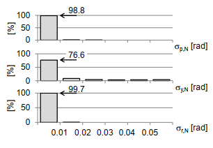Figure 8: Distribution of the pose variation detected in the used data.

6          Conclusions and Future Work

A novel method of monocular height estimation with 3DOF compensation of roll, pitch and yaw variations was proposed. The method can estimate height of objects with only two frames of a monocular camera. Experiments outdoors with the KITTI benchmark data (4997 frames and 436 objects) resulted in improved accuracy of the estimated heights from a maximum error of 1.51 m to 1.12 m and reduced number of estimation failures by 4 times, proving the validity and effectiveness of the proposed method. This method can be enhanced by improving monocular visual odometry techniques and considering translational variations of the camera during height estimation. Further investigation about influences of frame rate, moving velocity and robustness are planned in the future.

Conflict of Interest The authors declare no conflict of interest.

1. A. M. Kaneko, K. Yamamoto. Monocular Height Estimation by Chronological Correction of Road Unevenness. 2016 IEEE/SICE International Symposium on System Integration (SII2016). Sapporo, Japan. 2016. https://doi.org/10.1109/SII.2016.7843971
2. A. M. Kaneko, K. Yamamoto. Landmark Recognition Based on Image Characterization by Segmentation Points for Autonomous Driving. SICE Multi-Symposium on Control Systems 2016 (MSCS2016). Nagoya, Japan. 7-10 March, 2016. https://doi.org/10.1109/SICEISCS.2016.7470160
3. M. Aly. Real Time Detection of Lane Markers in Urban Streets. IEEE Intelligent Vehicles Symposium. Eindhoven. 4- 6 June, 2008. https://doi.org/10.1109/IVS.2008.4621152
4. T. Wu, A. Ranganathan. A Practical System for Road Marking Detection and Recognition. IEEE Intelligent Vehicles Symposium (IV). Alcala de Henares. 3-7 June, 2012. https://doi.org/10.1109/IVS.2012.6232144
5. P. Foucher, Y. Sebsadji and J. P. Tarrel, P. Nicolle. Detection and Recognition of Urban Road Markings Using Images. IEEE International Conference on Intelligent Transportation Systems (ITSC). Washington DC, USA. 2011. https://doi.org/10.1109/ITSC.2011.6082840
6. D. Scaramuzza. 1-Point-RANSAC Structure from Motion for Vehicle-Mounted Cameras by Exploiting Non-holonomic Constraints. International Journal of Computer Vision, Volume 95, issue 1, 2011. https://doi.org/10.1007/s11263-011-0441-3
7. M. W. Maimone, Y. Cheng, L. Matthies. Two years of Visual Odometry on the Mars Exploration Rovers. J. Field Robotics 24(3): 169-186 (2007). https://doi.org/10.1002/rob.v24:3
8. M. K. Momeni C. H. S. Diamantas, F. Ruggiero, and B. Siciliano. Height Estimation from a Single Cam- era View. In Proceedings of the International Conference on Computer Vision Theory and Applications (VISIGRAPP 2012)ISBN 978-989-8565-03-7, pages 358-364. DOI:
   10.5220/0003866203580364
9. P. Viswanath, I.A. Kakadiaris and S. K. Shah. A Simplified Error Model for Height Estimation using Single Camera. 2009 IEEE 12th International Conference on Computer Vision Workshops, ICCV Workshops. 2009. https://doi.org/10.1109/ICCVW.2009.5457466
10. N. Pears, B. Liang, Z. Chen. Mobile Robot Visual Navigation Using Multiple Features. EURASIP J. Adv. Sig. Proc. 2005(14): 2250-2259. 2005.
    https://doi.org/10.1155/ASP.2005.2250
11. A. Wedel, T. Schoenemann, T. Brox, D. Cremers. WarpCut – Fast Object Segmentation in Monocular Video. 29th DAGM Symposium, Heidelberg, Germany. Proceedings, pp. 264-273. 2007. http://doi.org/10.1007/978-3-540-74936-3 27
12. J. Campbell, R. Sukthankar et al. A Robust Odometry and Precipice Detection System Using Consumergrade Monocular Vision. Proceedings of the 2005 IEEE International Conference on Robotics and Automation, 2005. ICRA 2005. Pp 3421-3427. 2005. https://doi.org/10.1109/ROBOT.2005.1570639
13. S. Lovegrove, A. J. Davison, J. I. Guzman. Accurate Visual Odometry from a Rear Parking Camera. IEEE Intelligent Vehicles Symposium (IV). Pp 788-793. 2011. https://doi.org/10.1109/IVS.2011.5940546
14. N. Nourani-Vatani, et al. Practical Visual Odometry for Car-like Vehicles. IEEE International Conference on Robotics and Automation (ICRA). Kobe, Japan. 2009. https://doi.org/10.1109/ROBOT.2009.5152403
15. A. Geiger, P. Lenz and R. Urtasun. Are We Ready for Autonomous Driving? The KITTI Vision Benchmark Suite. Conference on Computer Vision and Pattern Recognition (CVPR). 2012. http://doi.org/10.1109/CVPR.2012.6248074
16. Bradski, G. Opencv. Dr. Dobbs Journal of Software Tools. 2000.
17. D.Nister. An Efficient Solution to the Five-Point Relative Pose Problem. IEEE Transactions on Pattern Analysis and Machine Intelligence, Vol. 26, No. 6. 2004. https://doi.org/10.1109/TPAMI.2004.17
18. E. Rosten, R. Porter and T. Drummond. FASTER and Better: A Machine Learning Approach to Corner Detection. IEEE Trans. Pattern Analysis and Machine Intelligence. 2010. https://doi.org/10.1109/TPAMI.2008.275
19. H. Hirschmuller. Accurate and Efficient Stereo Processing by Semi-Global Matching and Mutual Information. International Conference on Computer Vision and Pattern Recognition, 2005. https://doi.org/10.1109/CVPR.2005.56

(Click to view)

(Click to view)