Theoretical developments for interpreting kernel spectral clustering from alternative viewpoints

Introduction

In general, for classifying or grouping a set of objects (represented as data points) into subsets holding similar objects, the field of machine learning specifically, the pattern recognition- provides two great alternatives being essentially different fromeach other: Supervised- and Unsupervised-learning-based approaches. The former ones normally establish a model from beforehand known information on data normally provided by an expert, while the latter ones form the groups by following a natural clustering criterion based on a (traditionally heuristic) procedure of data exploration [1]. Therefore, unsupervised clustering techniques are preferred when object labelling is either unavailable or unfeasible. In literature, we can find tens of clustering techniques, which are based on different principles and criteria (such as: distances, densities, data topology, and divergences, among others) [2]. Some remarkable, emerging applications are inbalanced data analysis [3] and timevarying data analysis [4]. Particularly, spectral clustering (SC) is a suitable technique to deal with grouping problems involving hardly separable clusters. Many SC approaches have been proposed, among them: Normalized-cut-based clustering (NCC), which, applied as explained in [5], heuristically and iteratively estimates binary cluster indicators [5] or approximates the solution in a one-iteration fashion by solving a quadratic programming problem [6]. Kernel kmeans (KKM) that can be formulated using eigenvectors [7]. Kernel spectral clustering (KSC), which uses a latent variable model and a least-squares-supportvector-machine (LS-SVM) formulation [8]. This work has a particular focus on KSC, being one of the most modern approaches. It has been widely used in numerous applications such as time-varying data [9,10], electricity load forecasting [11], prediction of industrial machine maintenance [12], and among others. Also, some improvements and extensions have been proposed [12–14].

The aim of this work is to demonstrate the relationship between KSC and other approaches, namely NCC and KKM. To do so, elegant mathematical developments are performed. Starting from either the primal or dual formulation of KSC, we show clearly the links with the other considered methods. Experimentally, in order to assess the clustering performance, we explore the benefit of each considered method on image segmentation. In this connection, images extracted from the free access Berkeley Segmentation Data Set [15] are used. As a meaningful result of this work, Also, we provide mathematical and experimental evidence of the usability of combining together a LS-SVM formulation and a generic latent variable model for clustering purposes.

The rest of this paper is organized as follows: Section 2 outlines the primal-dual formulation for KSC starting with a LS-SVM formulation regarding a variable model, which naturally yields an eigenvector-

based solution. Sections 3 and 4 explore and discusses on the links of KSC with NCC and KKM, respectively. Some experimental results are shown in Section 5. Section 6 presents some additional remarks on improved versions of KSC and its relationship with spectral dimensionality reduction. Finally, section 7 draws some final and concluding remarks.

2 Kernel Spectral clustering

Accounting for notation and future statements, let us consider the following definitions: Define a set of N objects or samples represented by d-dimensional feature vectors. Likewise, consider a data matrix holding all the feature vectors, so that X ∈ R^N×d: X =

,…,x^⊤_N ]^⊤, where x_i ∈ R^d is the i-th d dimensional feature vector or data point. KSC is aiming to split X into K disjoint subsets, being K the number of desired groups.

2.1     Latent variable model and problem formulation

In the following, the clustering model is described. Let e^(l) ∈ R^N be the l-th projection vector, which is assumed in the following latent variable form:

                                     e(l) = Φw(l) +bl1N ,                                (1)

where w^(l) ∈ ^Rdh is the l-th weighting vector, b_l is a bias term, n_e is the number of considered latent variables, notation 1_N stands for a N dimensional all-ones vector, and the matrix Φ = [φ(x₁)^⊤,…,φ(x_N )^⊤]^⊤, Φ ∈ R^N×dh, is a high dimensional representation of data. The function φ(·) maps data from the original dimension to a higher one d_h, i.e., φ(·) : R^d → R^dh. Therefore, e^(l) represents the latent variables from a set of n_e binary cluster indicators obtained with sign(e^(l)), which are to be further encoded to obtain the K resultant groups.

From the least-squares SVM formulation of equation (1), the following optimization problem can be stated:

           max         1 Xn^e γ e                      − X^ne w(l)⊤w(l)          (2a)

l

        e(l),w(l),b(l) 2N                                    2

                                 l=1                                l=1

          s.t.e(l) = Φ⊤w(l) +bl1N ,                                                 (2b)

where γ_l ∈ R⁺ is the l-th regularization parameter and V ∈ R^N×N is a diagonal matrix representing the weight of projections.

2.2        Matrix problem formulation

For the sake of simplicity, we can express the primal formulation (2) in matrix terms, as follows:

                      tr(E^⊤VE tr(W^⊤W)            (3a)

E,W,b       2N                           2
s.t.E = ΦW+1N ⊗b⊤,	(3b)

where b = [b₁,…,b_ne ], b ∈ R^ne, Γ = Diag([γ₁,…,γ_ne]),

W    =      [w(1),··· ,w(ne)],       W       ∈ Rdh×ne,        and    E     =

[e⁽¹⁾,··· ,e^(ne)], E ∈ ^RN×ne. Notations tr(·) and ⊗ denote the trace and the Kronecker product, respectively. By minimizing the previous cost function, the goals of minimizing the weighting variance of E and maximizing the variance of W are reached simultaneously. Let ΣE be the weighting covariance matrix of E and Σ_W be the covariance matrix of W. Since matrix V is diagonal, we have that tr((V^1/2E)^⊤V^1/2E) = tr(ΣE). In other words, Σ_E is the covariance matrix of weighted projections, i.e., the projections scaled by square root of matrix V. As well, tr(W^⊤W) = tr(Σ_W). Then, KSC can be seen as a kernel, weighted principalcomponent analysis (KWPCA) approach [8].

2.3     Solving KSC by using a dual formulation

To solve the KSC problem, we form the corresponding Lagrangian of the problem from equation (2) as follows:

L(E,W,Γ,A) = tr(W^⊤W)

                                          −tr(A^⊤(E−ΦW−1_N ⊗b^⊤)),             (4)

where matrix A ∈ R^N×ne holds the Lagrange multiplier vectors A = [α⁽¹⁾,··· ,α^(ne)], and α^(l) ∈ R^N is the l-th vector of Lagrange multipliers.

Solving the partial derivatives on L(E,W,Γ,A) to determine the Karush-Kuhn-Tucker conditions, we obtain:

                       ∂^L       ⇒ E = NV−1AΓ−1,

                       ∂L     ⇒ W = Φ⊤A,

∂L

                                ⇒ E = ΦW,

                       ∂L     ⇒ b⊤1N = 0.

Therefore, by eliminating the primal variables from initial problem (2) and assuming a kernel trick such that ΦΦ^⊤ = Ω, being Ω ∈ ^RN×N a given kernel matrix, the following eigenvector-based dual solution is obtained:

                       AΛ = V(I_N +(1_N ⊗b^⊤)(ΩΛ)⁻¹)ΩA,                   (5)

where Λ = Diag(λ), Λ ∈ R^N×N, λ ∈ R^N is the vector of eigenvalues with λ_l = N/γ_l, λ_l ∈ R⁺.

b_l V1_N ).                       (6)Also, taking into account that the kernel matrix represents the similarity matrix of a graph with K connected components as well as V = D⁻¹ where D ∈ R^N×N is the degree matrix defined as D = Diag(Ω1_N ); then the K − 1 eigenvectors contained in A, associated to the largest eigenvalues, are piecewise constant and become indicators of the corresponding connected parts of the graph. Therefore, value n_e is fixed to be K − 1 [8]. With the aim of achieving a dual formulation, but satisfying the condition b^⊤1_N = 0 by centering vector b (i.e. with zero mean), the bias term should be chosen in the form

Thus, the solution of problem of equation (3) is reduced to the following eigenvector-related problem:

                                        AΛ = VHΩA,                                    (7)

where matrix H ∈ R^N×N is the centering matrix that is defined as

                           H N 1⊤_{N V1N}              N                     N ,V,

where I_N denotes a N-dimensional identity matrix and, Ω = [Ωij], Ω ∈ RN×N, being Ωij = K(xi,xj),i,j ∈

[N]. Notation K(·,·) : R^d × R^d → R stands for the kernel function. As a result, the set of projections can be calculated as follows:

                                     E = ΩA+1_N ⊗b^⊤.                                (8)

Once projections are calculated, we proceed to carry out the cluster assignment by following an encoding procedure applied on projections. Because each cluster is represented by a single point in the K − 1-dimensional eigenspace, such that those single points are always in different orthants due also to the KKT conditions, we can encode the eigenvectors considering that two points are in the same cluster if they are in the same orthant in the corresponding eigenspace [8]. Then, a code book can be obtained from the rows of the matrix containing the K − 1 binarized leading eigenvectors in the columns, by using sign(e^(l)). Then, matrix eE = sgn(E) is the code book being each row a codeword.

2.4        Out-of-sample extension

KSC can be extended to out-of-samples analysis without re-clustering the whole data to determine the assignment cluster membership for new testing data [8]. In particular, defining z ∈ R^ne as the projection vector of a testing data point x_test, and by taking into consideration the training clustering model, the testing projections can be computed as:

                                        z = A^⊤Ω_test +b,                                   (9)

where Ω_test ∈ R^ne is the kernel vector such that

Ω = [Ωtest1,…,ΩtestN ]⊤, test

and Ω_testi = K(x_i,x_test). Once, the test projection vector z is computed, a decoding stage is carried out that consists of comparing the binarized projections with respect to the codewords in the code book eE and assigning cluster membership based on the minimal Hamming distance [8].

2.5      KSC algorithm

Following the pseudo-code (Algorithm 1) to perform KSC is shown.

Algorithm 1 Kernel spectral clustering: [q_train,q_test] = KSC(X,K(·,·),K)

^1: Input: K, X, K(·,·)

^2: Form the kernel matrix Ω such that Ωij = K(y_i,x_j) ^3: Determine E through (8)

4: Form the training codebook by binarizing eE = sgn(E)

^5: Assign the output training labels q_train according to similar codewords

6: Compute the training codewords for testing

^7: Assign the output testing labels q_test according to the minimal Hamming distance when comparing with training codewords

^8: Output: qtrain,qtest

3 Linksbetween KSCandNCC

This section deals with the relationship between KSC and NCC, starting from the formulation of the NC problem until reaching a weighting principal component analysis (WPCA) formulation in a finite domain.

3.1     Multi-cluster      spectral            clustering (MCSC) from two point of view

In [5], the so-called Multi-cluster spectral clustering (MCSC) is introduced, which is based on the well-known k-way normalized cut-based formulation given by:

m(k)

(10a)

              K tr(M                                            =1        m

s.t. M ∈ {0,1}^N×K,               M1_K = 1_N .                                 (10b)

Expressions (10a) and (10b) are the formulation of the NC optimization problem, named (NCPM). Previous formulation can also be expressed as follows.

Let Ωb = D^−1/2ΩD^−1/2 be a normalized kernel matrix and L = D^1/2M be a binary matrix normalized by the square root of the kernel degree. Then, a new NCPM version can be expressed as:

                  1 tr(L⊤ΩL)                  1 PK          ℓ(k)⊤Ωℓ( )

                                 L          ℓ(k)

s.t.D−1/2L ∈ {0,1}N×K, D−1/2L1K = 1N , (11b) where ℓ^(k) is the column k of L.

Solution of former problem has been addressed in [5,16] by introducing a relaxed version, in which numerator is maximized subject to denominator is constant, so

          max                 Ω )            s.t.tr(L^⊤L) = const.            (12)

L

Indeed, authors assume the particular case L^⊤L = I_K, i.e. letting L be an orthonormal matrix. Then, solution correspond to any K-dimensional basis of normalized matrix eigenvectors. Despite that in [16] it is presented an one-iteration solution for NCPM with suboptimal results avoiding the calculation of SVD per iteration, the omitting of the effect of denominator tr(L^⊤L) by assuming orthogonality causes that the solution cannot be guaranteed to be a global optimum. In addition, this kind of formulation provide non-stable solutions due to the heuristic search carried out to determine an optimal rotation matrix [16].

3.2 Solving the problem by a difference: Empirical feature map

Recalling original problem 3.1, we introduce another way to solve the NCPM formulation via a minimization problem where the aims for maximizing tr(L^⊤ΩbL) and minimizing tr(L^⊤L) can be accomplished simultaneously, so:

                         maxtr(L^⊤ΩbLDiag(γ))−tr(L^⊤L)                 (13)

L where γ = (γ₁,…,γ_N )^⊤ is a vector containing the regularization parameters.

Let us assume Ω = ΨΨ^⊤ where Ψ is a N × N dimensional auxiliary matrix, and consider the following equality:

tr(Ωb) = tr(D^−1/2ΩD^−1/2) = tr(D⁻¹Ω)

= tr(D−1ΨΨ⊤) = tr(Ψ⊤D−1Ψ), then

D−1/2ΩD−1/2 = Ψ⊤D−1Ψ.

Previous formulation is possible since kernel matrix Ω is symmetric. Now, let us define h^(k) ∈ R^N = Ψ^⊤ℓ^(k) as the k-th projection and H = (h⁽¹⁾,··· ,h^(K)) as the projections matrix. Then, formulation given by (13) can be expressed as follows:

                               K                                                        K

         max               1 Xγ h(k)⊤Vh(k) − 1 Xℓ(k)⊤ℓ(k)              (14a)

k

        h(k),ℓ(k),γk 2K k=1                                2 k=1

        such that h^(k) = Ψℓ^(k),                                                  (14b)

where matrix V ∈ R^N×N can be chosen as:

• I_N: We can normalize matrix Ω in such way for all i condition P^N_j ω_ij = 1 is satisfied and therefore we would obtain a degree matrix equaling the identity matrix. Then, Ph^(l)⊤h^(l) = tr(H^⊤H), which corresponds to a PCA-based formulation.
• Diag(v): With v ∈ R^N such that v^⊤v = 1, we have a WPCA approach.
• D⁻¹: Given the equality V = D⁻¹, optimization problem can be solved by means of a procedure based on random walks; being the case of interest in this study.

3.2.1        Gaussian processes

In terms of Gaussian processes, variable Ψ represents a mapping matrix such that Ψ = (ψ(x₁),…,ψ(x_N )) and where ψ(·) : ^Rd → ^RN ) is mapping function, which provides a new N-dimensional data representation where resultant clusters are assumed to be more separable. Also, matrix Ω is to be chosen as a Gaussian kernel [17]. Therefore, according to optimization problem given by (14), term h^(k) is to be the k-th projection of normalized binary indicators as h^(k) = Ψℓ^(k).

3.2.2        Eigen-solution

We present a solution for 14, which after solving the KKT conditions on its corresponding Lagrangian, an eigenvectors problem is yielded. Then, we first solve the Lagrangian of problem (14) so:

L(h,ℓ,γ,α) = Vh

where α is a N-dimensional vector containing the Lagrange multipliers.

Solving the partial derivatives to determine the KKT conditions, we have:

                               ∂^L                            K

                                     ⇒ h Dα,

                               ∂L                               ⊤

                                = 0        ⇒ ℓ = Ψ α,

∂ℓ
∂L = 0	⇒ h = Ψℓ.

∂α

Eliminating the primal variables, we obtain the following eigenvector problem:

                                         λα = D⁻¹Ωα,                                  (16)

where λ = N/γ. Then, matrix ∆_K = (α⁽¹⁾,··· ,α^(K)) can be computed as the eigenvectors associated with the first K longest eigenvalues of D⁻¹Ω.

Finally, projections matrix H is in the form

                             H = ΨL = ΨD^1/2M = Ω∆_K,                      (17)

and therefore M = Ψ⁻¹D^−1/2Ω∆_K, where Ψ can be obtained from a Cholesky decomposition.

Then, within a finite domain, both solution and formulation of NCC can be expressed similarly as done in KSC. So it is demonstrated the relationship between a kernel-based model and Gaussian processes.

4 Links between KSC andKKM

Kernel K-means method (KKM) is a generalization of standard K-means that can be seen as a spectral relaxation when introducing a mapping function in the objective function formulation [18]. As mentioned throughout this paper, spectral clustering approaches usually are performed on a lowerdimensional space, keeping the pairwise relationships among nodes. Then, it often leads to a relaxed NPproblems where continuous solutions are obtained by a eigen-decomposition. Such an eigen-decomposition is regarding the normalized similarity matrix (Laplacian, as well). In a Kernel K-means framework, eigenvectors are considered as geometric coordinates and then K-means methods is applied over the eigen-space to get the resultant clusters [19,20].

Previous instance is as follows: Suppose that we have a gray scale matrix m × n pixels in size. Characterizing each image pixel with d features -e. g., color spaces, morphological descriptors- it is yielded as a result a data matrix in the form X ∈ R^N×d, where N = mn. Afterwards, the eigenvectors VR^N×N of a normalized kernel matrix P ∈ ^RN×N such that P = D⁻¹Ω, being Ω the kernel matrix and D ∈ R^N×N the corresponding degree matrix. Then, we proceed to cluster V into K groups using K-means algorithm: q = kmeans(V,K), being q ∈ R^N the output cluster indicator such that q_i ∈ [K]. The segmented image is then a m × n sized matrix holding regions in accordance with q.

Briefly put, one simple way to perform a KKM procedure is applying k-means over the eigen-space. In Equation (7), the dual formulation is regarding the matrix S = VHΩ where weighting matrix can be chosen as V = D⁻¹ and D is the degree of the data-related graph. Since H causes a centering effect, matrix S is the same as P when kernel matrix Ω is centered. In other words, KKM can be seen as a KSC formulation with an incomplete latent variable model being a noncentered one (with no bias term).

5 Results anddiscussion

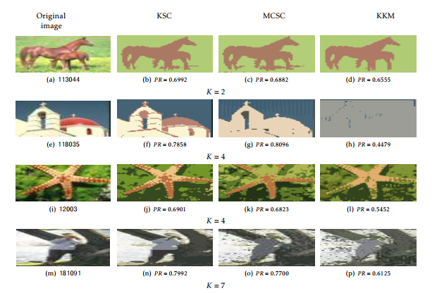
In order to show how considered methods work, we conduct some experiments to test their clustering ability on segmenting images. To do so, the segmentation performance is quantified by a supervised index noted as Probabilistic Rand Index (PR), explained in [21], such that PR ∈ [0,1], being 1 when regions are properly segmented. Images are drawn from the free access Berkeley Segmentation Data Set [15]. To represent each image as a data matrix, we characterize the images by color spaces (RGB, YCbCr, LAbB, LUV) and the xy position of each pixel. At the end, data matrix X gathers N pixels represented by d characteristics (variables). To run the experiment, we resize the images at 20% of the original size due to memory usage restrictions. All the methods are performed with a given number of clusters K manually set as shown in shown in Fig. 5 and using the scaled exponential similarity matrix as described in [19], setting the number of neighbors to be 9.

To test all the methods in a fair scenario, kernelbased methods (KSC and KKM) use Ω as kernel matrix, whereas such a matrix is the affinity matrix for NCC. As well, to perform the clustering procedure, the number of clusters is the same for all the considered methods. As can be readily appreciated, KSC overcome the rest of studied clustering methods. This fact can be attributed to the KSC formulation, which involves a whole latent variable model being in turn incorporated within a LS-SVM framework. Indeed, just like principal component analysis (PCA), KSC optimizes an energy term. Differently, such an energy term is regarding a latent variable instead of directly the input data matrix. Concretely, a latent variable model is used, which is linear and formulated in terms of projections of the input data. The versatility of KSC relies on the kernel matrix required during the optimization procedure of its cost function. Such a matrix holds pairwise similarities, then KSC can be seen as data-driven approach that not only consider the nature of data but yields a true clustering model. It is important to quote that -depending on the difficulty of the segmentation task- data matrices representing images yield features spaces, which may present hardly separable classes. Then, we have demonstrated the benefit of the KSC approach that uses a model along with a LS-SVM formulation -everything within a primal-dual scheme. Other studies have also proven the usability and versatility of this kind of approaches [8,22].

6 Additionalremarks

As explained in [23], KSC performance can be enhanced in terms of cluster separability by optimally projecting original input data and performing the clustering procedure over the projected space. Given the unsupervised nature, spectral clustering becomes very often a parametric approach, involving then a stage of selection/tunning of collection of initial parameters to avoid any local-optimum solution. Typically, the initial parameters are the kernel or similarity matrix and the number of groups. Nonetheless, in some problems when data are represented in a high-dimensional space and/or data-sets are nonlinearly separable, a proper feature extraction may be an advisable alternative. In particular, a projection generated by a proper feature extraction procedure may provide a new feature space wherein the clustering procedure can reach more accurate cluster indicators. In other words, data projection accomplishes a new representation space, where the clustering can be improved, in terms of a given mapping criterion, rather than performing the clustering procedure directly over the original input data.

Figure 1: Clustering performance on image segmentation reached by all the considered methods. It is noticeable that KSC overcome the remaining methods. Images are data that traditionally involve highly nonseparable clusters. Therefore, the benefit of using a whole latent variable model within a LS-SVM formulation

The work developed in [23] introduces a matrix projection focusing on a better analysis of the structure of data that is devised for a KSC. Since data projection can be seen as a feature extraction process, is verified.

we propose the M-inner product-based data projection, in which the similarity matrix is also considered within the projection framework, similarly as discussed in [24]. There are two main reasons for using data projection to improve the performance of kernel spectral clustering: firstly, the data global structure is taken into account during the projection process and, secondly, the kernel method exploits the information of local structures.

Another study [25] explores the links of KSC with spectral dimensionality reduction from a kernel viewpoint. Particularly, the proposed formulation is LSSVM in terms of a generic latent variable model involving the projected input data matrix. In order to state a kernel-based formulation, such a projection maps data onto a unknown high-dimensional space. Again, the solution of the optimization problem is addressed through a primal-dual scheme. Finally, once latent variables and parameters are determined, the resultant model outputs a versatile projected matrix able to represent data in a low-dimensional space. To do so, since the optimization is posed under a maximization criterion and dual version has a quadratic from, the eigenvectors associated with the largest eigenvalues can be chosen as a solution. Therefore, the generalized kernel model may represente a weighted version of kernel principal component analysis.

7 Conclusions

This works explores a widely-recommended method for unsupervised data classification, namely kernel spectral clustering (KSC). From elegant developments, the relationship between KSC and two other well-known spectral clustering approaches (normalized cut clustering and kernel k-means) is demonstrated. As well, the benefit of KSC-like approaches is mathematically and experimentally proved. The goodness of KSC relies on the nature of its formulation, which is based on a latent variable model incorporated into a least-square-support-vector-machine framework. Additionally, some key aspects and hints to improve KSC performance as well as its ability to represent dimensionality reduction approaches are briefly outlined and discussed.

As a future work, a generalized clustering framework is to be designed so that a wide range of spectral approaches can be represented. Doing so, the task of selecting and/or testing a spectral clustering method would become easier and fairer.

1. F. Schwenker and E. Trentin, “Pattern classification and clustering: a review of partially supervised learning approaches,” Pattern Recognition Letters, vol. 37, pp. 4–14, 2014.
2. A. K. Jain, “Data clustering: 50 years beyond k-means,” Pat-tern recognition letters, vol. 31, no. 8, pp. 651–666, 2010.
3. S. Belarouci and M. A. Chikh, “Medical imbalanced data classification,” Advances in Science, Technology and Engineering Systems Journal, no. 3, pp. 116–124.
4. H. Chebi, D. Acheli, and M. Kesraoui, “Dynamic detection of abnormalities in video analysis of crowd behavior with DB-SCAN and neural networks,” Advances in Science, Technology and Engineering Systems Journal, no. 5, pp. 56–63.
5. Y. S. X. and S. Jianbo, “Multiclass spectral clustering,” in ICCV ’03: Proceedings of the Ninth IEEE International Conference on Computer Vision. Washington, DC, USA: IEEE Computer Society, 2003, p. 313.
6. D. H. Peluffo-Ordóñez, C. Castro-Hoyos, C. D. Acosta-Medina, and G. Castellanos-Domínguez, “Quadratic problem formulation with linear constraints for normalized cut clustering,” in Iberoamerican Congress on Pattern Recognition. Springer, 2014, pp. 408–415.
7. I. S. Dhillon, Y. Guan, and B. Kulis, “Kernel k-means: spectral clustering and normalized cuts,” in Proceedings of the tenth ACM SIGKDD international conference on Knowledge discovery and data mining. ACM, 2004, pp. 551–556.
8. C. Alzate and J. A. K. Suykens, “Multiway spectral clustering with out-of-sample extensions through weighted kernel pca,” Pattern Analysis and Machine Intelligence, IEEE Transactions on, vol. 32, no. 2, pp. 335–347, 2010.
9. D. H. Peluffo-Ordóñez, S. García-Vega, A. M. Alvarez-Meza, and C. G. Castellanos-Domínguez, “Kernel spectral clustering for dynamic data,” in Iberoamerican Congress on Pattern Recognition. Springer, 2013, pp. 238–245.
10. R. Langone, C. Alzate, and J. A. Suykens, “Kernel spectral clustering with memory effect,” Physica A: Statistical Mechanics and its Applications, 2013.
11. C. Alzate and M. Sinn, “Improved electricity load forecasting via kernel spectral clustering of smart meters,” in 2013 IEEE 13th International Conference on Data Mining. IEEE, 2013, pp. 943–948.
12. R. Langone, R. Mall, C. Alzate, and J. A. Suykens, “Kernel spectral clustering and applications,” in Unsupervised Learning Algorithms. Springer, 2016, pp. 135–161.
13. D. H. Peluffo-Ordóñez, C. Alzate, J. A. K. Suykens, and G. Castellanos-Domínguez, “Optimal data projection for kernel spectral clustering,” in European Symposium on Artificial Neural Networks, Computational Intelligence and Machine Learning, 2014, pp. 553–558.
14. S. Mehrkanoon, C. Alzate, R. Mall, R. Langone, and J. A. Suykens, “Multiclass semisupervised learning based upon kernel spectral clustering,” IEEE transactions on neural net-works and learning systems, vol. 26, no. 4, pp. 720–733, 2015.
15. D. Martin, C. Fowlkes, D. Tal, and J. Malik, “A database of human segmented natural images and its application to evaluating segmentation algorithms and measuring ecological statistics,” in Proc. 8th Int’l Conf. Computer Vision, vol. 2, July 2001, pp. 416–423.
16. D. Peluffo, C. D. Acosta, and G. Castellanos, “An improved multiclass spectral clustering based on normalized cuts,” XVII Iberoamerican Congress on Pattern Recognition – CIARP, 2012.
17. C. Rasmussen and C. Williams, Gaussian processes for machine learning. MIT press Cambridge, MA, 2006, vol. 1.
18. H. Zha, C. Ding, M. Gu, X. He, and H. Simon, “Spectral relaxation for k-means clustering,” Advances in neural information processing systems, vol. 14, pp. 1057–1064, 2001.
19. L. Zelnik-manor and P. Perona, “Self-tuning spectral clustering,” in Advances in Neural Information Processing Systems 17. MIT Press, 2004, pp. 1601–1608.
20. I. S. Dhillon, Y. Guan, and B. Kulis, “Kernel k-means, spectral clustering and normalized cuts,” 2004.
21. R. Unnikrishnan, C. Pantofaru, and M. Hebert, “Toward objective evaluation of image segmentation algorithms,” Pattern Analysis and Machine Intelligence, IEEE Transactions on, vol. 29, no. 6, pp. 929–944, 2007.
22. D. H. Peluffo-Ordóñez, J. A. Lee, and M. Verleysen, “Generalized kernel framework for unsupervised spectral methods of dimensionality reduction,” in Computational Intelligence and Data Mining (CIDM), 2014 IEEE Symposium on. IEEE, 2014, pp. 171–177.
23. D. H. Peluffo-Ordóñez, C. Alzate, J. A. Suykens, and G. Castellanos-Domínguez, “Optimal data projection for kernel spectral clustering.” in European Symposium on Artificial Neural Networks – ESANN, 2014.
24. J. Rodríguez-Sotelo, D. Peluffo-Ordóñez, D. Cuesta-Frau, and G. Castellanos-Domínguez, “Unsupervised feature relevance analysis applied to improve ecg heartbeat clustering,” Computer Methods and Programs in Biomedicine, 2012.
25. X. Blanco-Valencia, M. Becerra, A. Castro-Ospina, M. Ortega-Adarme, D. Viveros-Melo, J. Alvarado-Peréz, and D. Peluffo-Ordóñez, “Kernel-based framework for spectral dimensionality reduction and clustering formulation: A theoretical study,” ADCAIJ: Advances in Distributed Computing and Articial Intelligence Journal, 2017.

(Click to view).

(Click to view).