1. Introduction

Sensor fault detection and diagnosis has been a research topic for decades, and many articles have been published. Interested readers are referred to the survey paper by Frank [16]. While fault detection is relatively easy, isolation of multiple faults is still a challenge to many existing schemes.  This paper proposes a novel and systematic approach to sensor and actuator integrity monitoring in systems such as jet engine of an aircraft. The first part is a fault detection scheme that can detect the presence of both sensor and actuator failures with maximized sensitivity. The newly proposed approach is based on analytic redundancy, which means no additional redundant sensors are needed. System input-output relationships (state-space dynamical model of the system) are used to help differentiate different sensor and actuator failures. The second step in the proposed scheme is the fault isolation. A proven technique known as contribution analysis [17-18] that has been widely used in process control industry is utilized for root cause search of sensor faults. Contribution analysis is a practical technique for fault isolation, particularly useful for multiple faults. Moreover, the concept of the structured residuals [19] is applied for actuator fault isolation. Finally, in line with the fault isolation results, a systematic procedure is conducted to reconstruct the faulty sensors/actuators such that the considered system, e.g., an aircraft, can keep functioning with acceptable performance in presence of sensor and/or actuator failures. Extensive simulations using a jet engine model clearly demonstrated the correctness and effectiveness of the proposed algorithms.Sensors and actuators are critical components in complex systems. For instance, in an airplane, effective flight control is impossible if sensors and/or actuators are malfunctioning [1-9]. Sensors and actuators can fail, and their failures have a significant impact on the performance of a system. In some applications such as arcing detection in power network [10] and motor corona monitoring [11], sensor and actuator condition plays critical role.   In the worst case, the failure even can affect safe operation of the system, leading to a catastrophic event. Sensor failures may include precision degradation, drift, frozen reading, and complete failure [12]. Similarly, actuator failures may include limited range of motion, e.g., valve stiction, and complete failure [13]. It is a challenging task to detect sensor and actuator failures [1-5, 14-15] because sensor outputs contain information from a multitude of sources: normal system outputs, faulty sensor signals, and signals due to noise and external disturbances. Isolating different signals requires utilization of the input-output relationship of the system. Conventional approaches to increasing reliability of aircraft systems include installing redundant sensors, which will add more weights, costs, complexity, and most importantly, additional reliability problems.

We would like to mention that this paper is an expanded version of our earlier work [20]. More details and simulations have been added to enrich the technical contents. The paper is organized as follows. Section II describes the problem formulation by introducing notations and terminologies. Section III, IV, and V summarize the fault detection, fault isolation, and fault reconstruction algorithms. Section VI includes simulation results of applying the proposed algorithms towards a jet engine. Finally, conclusions are drawn in Section VII and future work is discussed.

2.       Problem formulation

Consider the following dynamical system with multiple inputs (MI) and multiple outputs (MO),

where  is the state variable vector,  the input vector, and  the output vector, at time ;  are system matrices with compatible dimensions;  and  are process disturbance and measurement noise, respectively. It is assumed that  and  are independent random variables with zero mean values and covariance matrices

     It is further assumed that ,  and  are known because they can be either derived or identified from historical data by using the subspace method of identification [21].

Note that (1) represents a failure-free MIMO system. In the presence of sensor failures,  and actuator failures  one has

For a system represented by (2), given available data , it is expected to detect if the magnitude of

is non-zero.  If the answer is yes, the magnitude is estimated and

the failure direction matrix   is identified.  Finally, the

failed sensors or actuators will be reconstructed on-line and in real time such that all the sensors are always functional with accepted performance. Herein, it must be addressed that  comes from controllers. Therefore, it is always available and does not include any actuator failures. On the other hand,  is measured, also always available, and can contain sensor failures. The variables and terms in this paper are summarized in Appendix.

3.       Detection of Faulty Sensors/Actuators

Given an integer  (its determination will be discussed later), performing an algebraic manipulation on (2) leads to

where  Note that at ,

Define a stacked vector

Similarly, define five more stacked vectors

It turns out from (3)-(6) that

where

 Herein, the choice of  is discussed. It must be chosen such that  There can be many candidates for  to meet such a requirement. We just select a proper value that allows us to perform both fault detection and isolation. This will be elaborated later.

       With the establishment of (7), a primary residual vector (PRV) can be calculated for fault detection. Select a matrix  from the null space of . Multiplying both sides of (7) by  leads to

where  has been considered.

as the PRV for fault detection due to the following facts:

1. In the ideal case, i.e., no fault, no noise, and no disturbance,
2. Without any faults, is a moving average (MA) process of noise vectors and , having zero mean value and covariance matrix

where    with  being an identity matrix and  the Kronecker tensor product [30].

1. In the presence of sensor and/or actuator faults, the PRV is

which is a random vector with non-zero mean,

and covariance [22]. Therefore, fault detection is to check if the mean value of the PRV is zero.

So far, no discussion on the calculation of has been conducted yet. Considering the dimension and rank of , it can be figured out that  has  rows and columns. Detailed steps to calculate , which are lengthy but straightforward, are documented in [19].

Assume that  and   are Gaussian distributed. It can be easily shown that  follows a zero mean Gaussian distribution with an identity covariance matrix [22]. Therefore, define

as the fault detection index, which follows a distribution with degree of freedom  [22]. With a pre-determined confidence limit, if   exceeds the limit, it indicates that some sensors and or actuators are faulty. Otherwise, everything is normal.

At the end of this section, the issue of disturbance decoupling is discussed. It has been assumed that  is Gaussian distributed. In reality, this assumption sometimes may be not valid. If this is the case, one can try to decouple the effect of disturbance as much as possible.

Note that in the PRV represented by (9), the disturbance contributed term is  Perform a singular value decomposition (SVD) on  and design  such that each of its rows is orthogonal to the principal left singular vectors related to few largest singular values of   As a consequence, effect of  can be decoupled partially. How much percentage of  can be decoupled? This depends on the dimension of  and the rank of  Intuitively, the lower the rank of is, the easier to decouple  from the PRV. Even if  cannot be removed from the PRV completely, it can be decoupled to some extent by using the above-mentioned SVD [23].

4.       Isolation of Faulty Sensors/Actuators

   While many methods have been available, here contribution analysis [18] is proposed for sensor fault isolation due to its practicality and simplicity. Computationally, the PRV is , which is contributed by  and . In the presence of sensor faults, the PRV will deviate from its nominal values. Consequently, by analyzing the contributions in  from each element of , the faulty sensors can be identified.

However, since  does not include any actuator failures, contribution analysis cannot be used for isolation of actuator failures. We will propose the structured residual-based approach towards actuator fault isolation. Therefore, combining contribution analysis [17-18] and the structured residual-based approach [19] will develop a comprehensive fault isolation methodology for both sensor and actuator failures.

4.1. Contribution Analysis for Isolation of Faulty Sensors

We illustrate how to identify faulty sensors by contribution analysis first.  It turns out from (5) and the first line of (9) that

Table 1. Incidence matrix showing actuator fault isolation logic.

where  is the  column of matrix  and  is the  element of stacked vector .

     If the  sensor has a failure for any , the failure-associated term in  is a vector:

Moreover, define

where  is the scaled counterpart of , i.e., mean-centered and divided by its standard deviation.

If a sensor failure begins to occur at time instance  and ends at , then one calculates the absolute average value, i.e.,

for all , obtaining  magnitude values.

 Any sensor that has the largest magnitude defined by (13) can be identified as faulty. For example, if Sensor 5 has the largest magnitude, then it can be inferred that it is faulty. As a result, the

failure direction matrices for the sensor is .

4.2. Isolation of Faulty Actuators

In order to isolate faulty actuators, one can also generate a set of structured residual vectors (SRVs) in line with a predetermined isolation logic [18]. For simplicity, assume that at each time, only a single actuator can be faulty. Under this assumption, for the system represented by (2), we design a set of   SRVs such that the  SRV is insensitive to the  actuator fault, while of maximized sensitivity to faults in other actuators for . Sensitivity of all the designed  SRVs to actuator faults can be described by the following incidence matrix shown in Table 1.

In the above incidence matrix shown in Table 1, ‘0’/‘1’ means insensitivity/maximized sensitivity of a SRV to an actuator fault. For instance, in presence of a fault, if  is not affected by the fault, while all the other SRVs are affected, then the  actuator is faulty.

Mathematically, the  SRV can be calculated by

where  is fault free, and the matrix  is designed such that  and the following associated

are excluded from . This indicates that

for all . Design of   is documented in [19]. Similar to (11),

is defined as the actuator fault isolation index, where  is the covariance of  for .

At the end of this section, hereafter we summarize the steps to perform detection and isolation of sensor and actuator faults:

6. Develop an isolation logic under an assumed fault pattern.
7. Design the PRV and a set of SRVs in line with the pre-determined isolation logic.
8. From a set of training data, calculate a sequence of PRV and sequences of SRVs. Calculate their respective thresholds.
9. Check if the detection index given by (11) is triggering an alarm.
10. Use contribution analysis to isolation sensor faults.
11. Use the SRVs to isolate actuator faults.

The above procedures are detailed also in the following flow chart. We divide the procedures into off-line, which is the preparation phase, and the online parts.

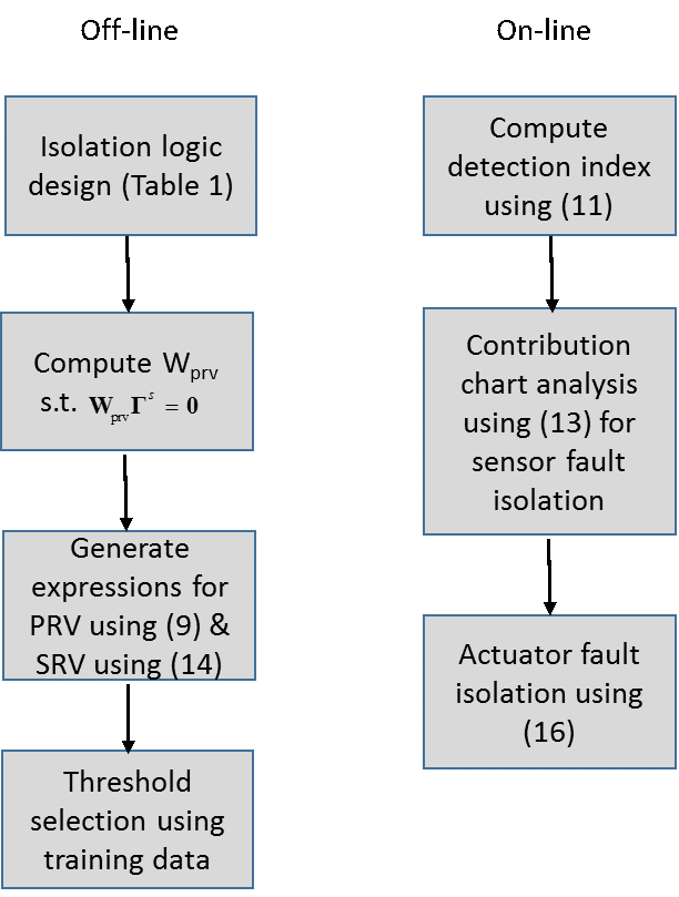Figure 1. Off-line and online procedures.

5.       Reconstruction of Faulty Sensors and Actuators

After identification of faulty sensors/actuators, one has to estimate the fault magnitudes first. Then, from the estimated fault value, faulty sensors can be reconstructed.

5.1.  Estimation of Fault Magnitudes

It can be derived from

With known  and  in line with [12], one can estimate  by minimizing

giving

If the matrix   is of full rank, one can get the least squares (LS) solution to  easily. If the matrix is of rank deficiency, one can apply a latent variable-based approach, such as the partial least squares (PLS), to estimate the fault magnitude [24].

 5.2.        Reconstruction of Faulty Sensors

 

   With estimated fault magnitudes, one can correct measurements of the faulty sensors. The measurements in faulty sensors are affected both by and  In order to get the corrected measurements in faulty sensors, one can design a Kalman filter,

where  is the corrected measurement of faulty sensors.

6.       Numerical Examples

The proposed methodology for sensor/actuator fault detection, isolation, and reconstruction is applied to a gas turbine jet engine control system [25].

6.1.  The Simulated System

The gas turbine engine can be described essentially as a heat engine that uses atmospheric air as a working medium to generate propulsive thrust and mechanical power. The central unit of the mechanical arrangement comprises two main rotating parts, the compressor and the turbine. The control system has the function of coordinating the main burner fuel flow and the propelling exhaust nozzle.

The thermodynamic model of the engine is in continuous-time domain. It has 17 state variables, including pressures, air and gas mass flow rates, shaft speeds, absolute temperatures, and static pressure. This is a highly nonlinear dynamic structure that has grossly different steady-state operation over the entire range of spool speeds, flow rates, and nozzle areas. The linearized 17^th model in the continuous-time domain is used here for study. The nominal operating point is set at 70% of the demand high spool speed ( ). For practical reasons and convenience of design, a fifth-order model is employed [25] to approximate the 17th-order model as represented by (20), where a sampling period of s was taken.

Using a reduced-order model to approximate the full-order dynamic system leads to modeling errors. Another problem is that the operating point of the system varies according to realistic running conditions. In general, different operating points correspond to different plant models. In the practical situation, the design of the fault detection and isolation scheme is based on a fixed mode. When the operating point changes, a model-plant mismatch occurs. Therefore, the system is represented by a fifth order state space model with two inputs, five outputs, and disturbance, i.e.

where the two inputs are main engine fuel flow rate and the exhaust nozzle area. In addition, the five outputs are compressor shaft speed, two pressure measurements, two temperature measurements, and the demand high spool speed. In addition,   represents the afore-mentioned modeling errors or model plant mismatch and  is measurement noise. It is assumed that and  are independently distributed Gaussian white noise sequences, with respective covariance matrices  and

Given the model parameters, selecting we calculate the following matrices       , and  in line with the formulas in (7).

We then calculate the matrix, , to generate the PRV for fault detection. In accordance with [19],  is calculated such that each of its rows is orthogonal to  while having maximized covariance with the non-zero singular value related-left singular vectors of

   With the calculated , the PRV is generated by

                .

Furthermore, we calculate two more matrices   and  to generate two SRVs

for   according to the isolation logic listed in Table 1.

Without any faults, we used (20) to generate 10,000 samples of training data, where , and accordingly we calculated three sequences of , , and , respectively. Using such sequences, we estimated the covariance,   of , , and .

We calculated a sequence of fault detection index  from  and  by using (11). It is depicted below with a confidence limit  (the red line in the graph). Moreover, we calculated two sequences of , which are depicted in Figure 2, respectively, with their own confidence limits.

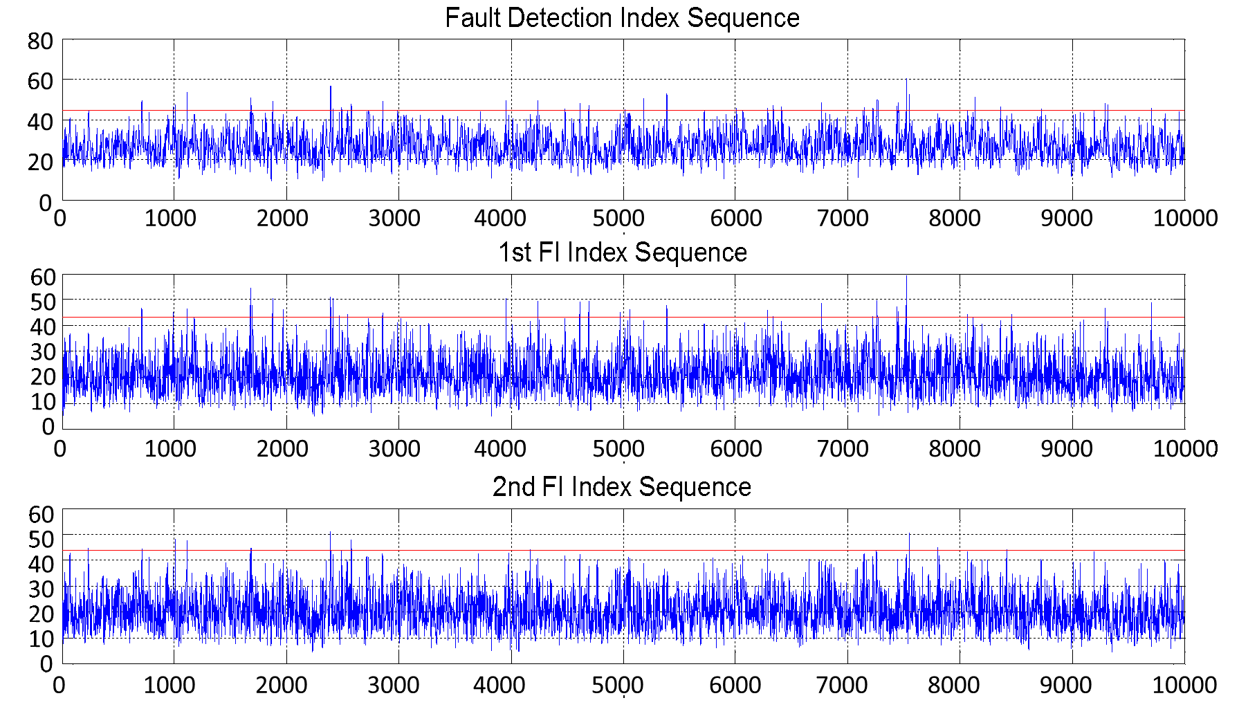Figure 2.  Fault detection and Isolation indices from training data.

It must be mentioned that the method proposed by [16] is used to determine the confidence limit of  given a level of confidence 99%. And such a limit will be employed for fault detection in test data.

6.2.  Generation of Test Data and FDI Results

    Many case studies have been conducted, and few results are presented hereafter.

6.2.1 Case 1: Detection and Isolation of a Faulty Actuator

A time varying fault simulated by

is introduced to one actuator, where

and . Note that  denotes the instant at which a fault begins to occur.  In this case, the test data are generated from the following equation:

where as selected before.

From available data sequences , we generated the PRV and two SRVs. At the meanwhile, we calculated the fault detection index sequence  and two fault isolation index sequences and  As clearly shown in Figure 3, as time goes by,  exceeded its limit, indicating that a fault/faults has/have occurred.

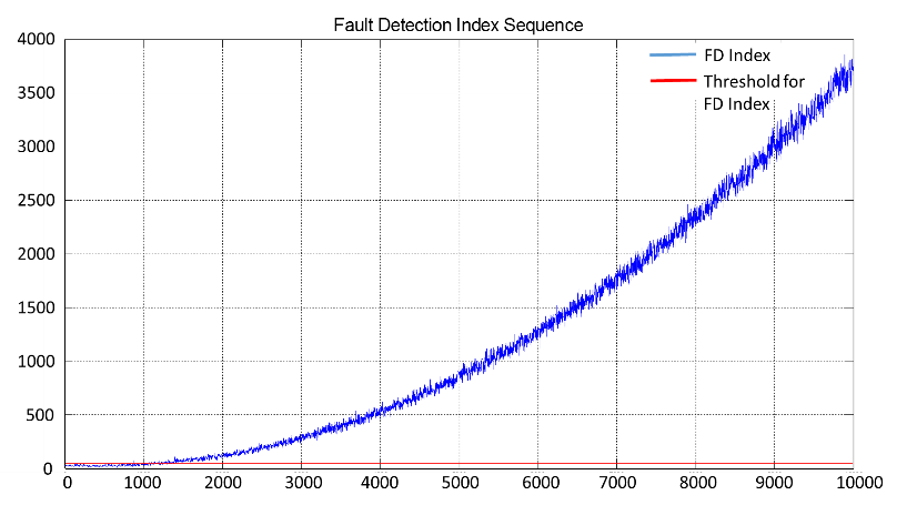Figure 3.  Fault Detection Result from Test Data.

Having detected the fault, we investigated the isolation of faulty sensors/actuators based on data collected from, e.g., sample 510 until sample 804. The contribution analysis bar chat is shown in Figure 4. From the bar chart, it is hard to infer anything, because the bar magnitudes from all sensors are very close.

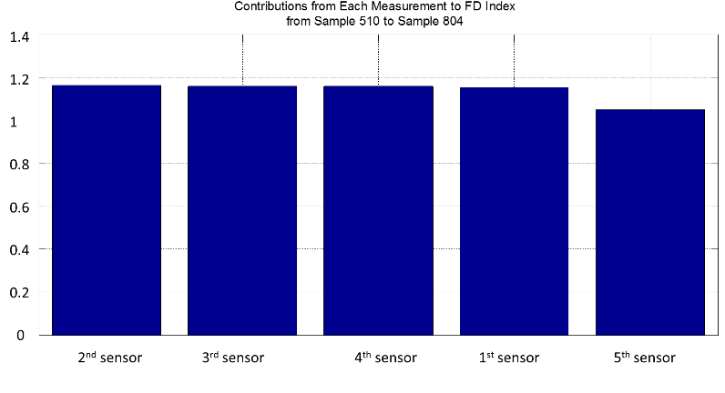Figure 4.  Contribution Analysis Results.

   The first isolation index sequence is illustrated in Figure 5, which is not affected by the fault at all. Furthermore, the second fault isolation index sequence is shown in Figure 6. In this figure, the sequence is beyond its limits after the fault happened. Therefore, in terms of the pre-determiend isolation logic, it can be inferred that the first actuator is faulty. At last, the estimated fault value is depicted in Figure 7.

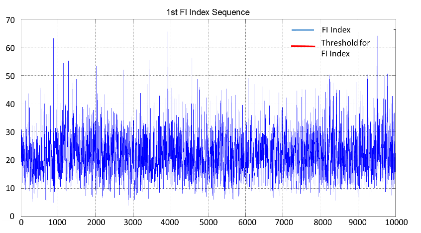Figure 5.  The 1^st Fault Isolation Index Sequence Calculated from Test Data.

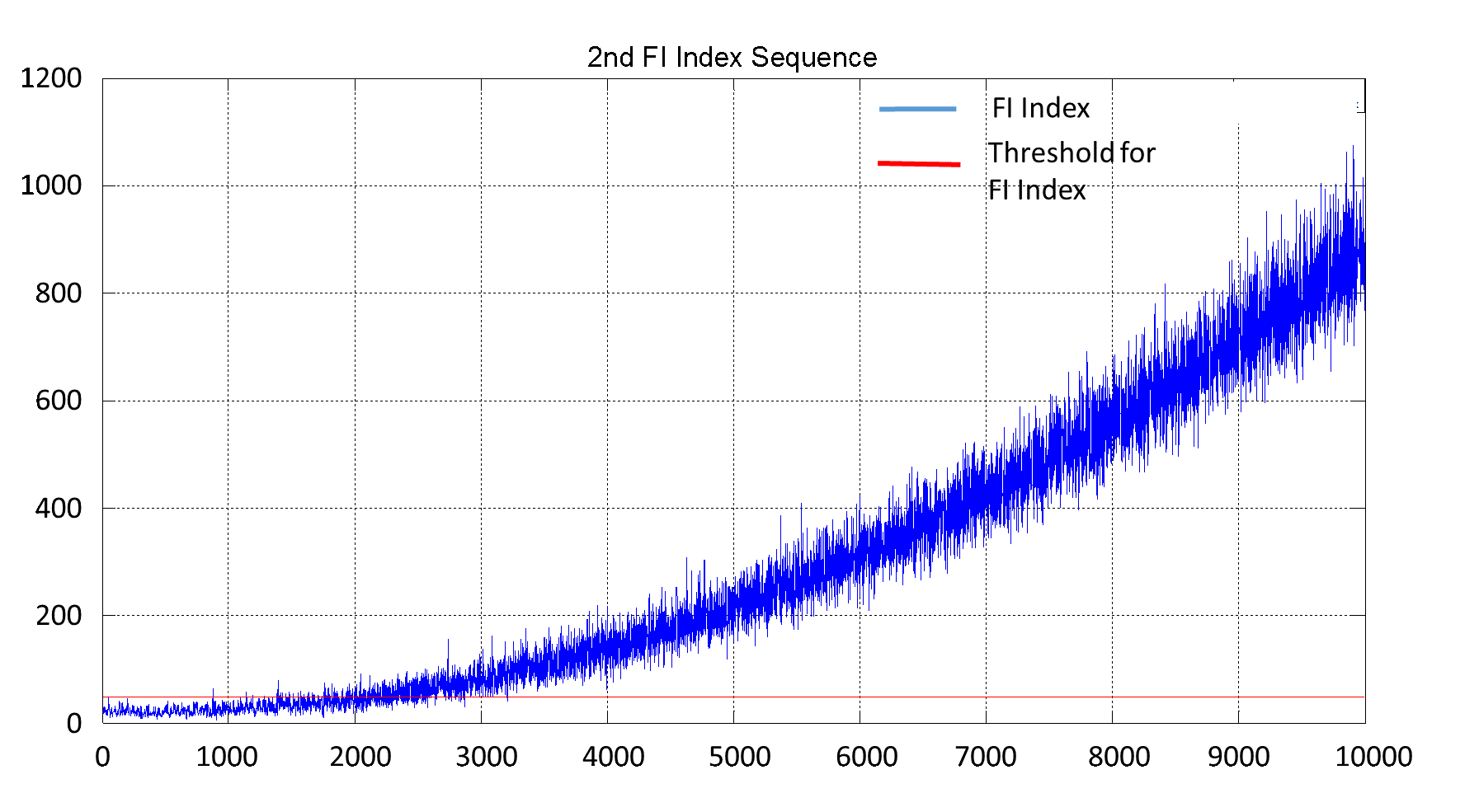Figure 6. The 2^nd Fault Isolation Index Sequence Calculated from Test Data.

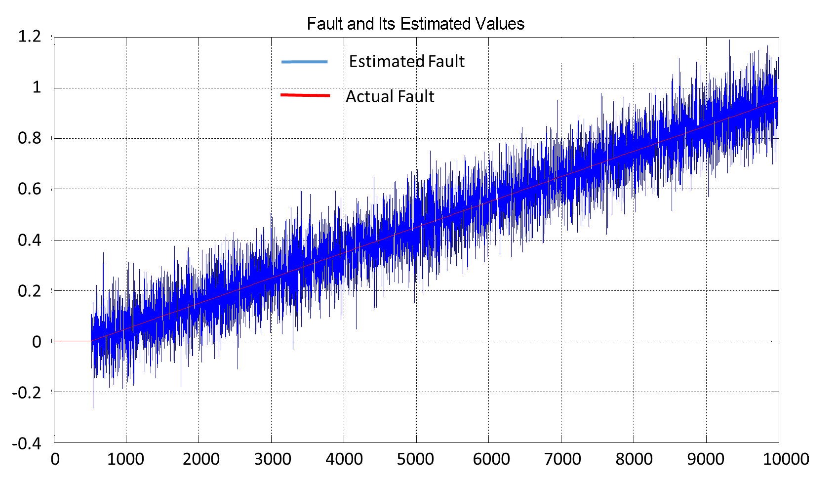Figure 7. Actual and Estimated Fault Values from Test Data.

6.2.2  Case 2: Detection and Isolation of a Faulty Sensor

     A bias with size 1.5 was introduced to a sensor. The fault detection index is displayed in Figure 8, where the exceeds its limit at sample 3000, giving .

Having detected the sensor fault, the next step is to isolate the faulty sensor by conducting the contribution analysis. A bar chart showing the contributions from all five sensors is depicted in Figure 9, where  and .

    It is clearly shown that the first output has made the most significant contribution to the sensor failure. Therefore, it can be inferred that the first sensor is faulty.

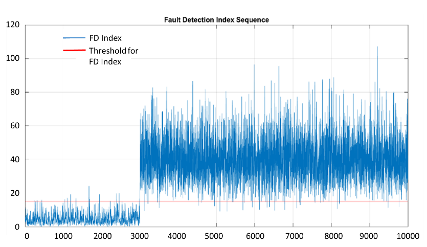Figure 8. Detection result of a sensor fault

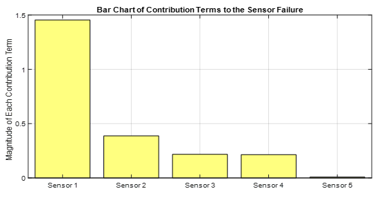Figure 9. Contribution analysis result of a sensor failure

6.2.3  Case 3: Detection and Isolation of Multiple Faulty Sensors

    The simulated system has five sensors in total. Assume that each sensor has a reliability of , then one can calculate the probabilities of simultaneous sensor failures.  The results are listed in Table 2.  For example, the probability that  sensors are faulty simultaneously is

where   is the combination of  from 5 for .

Table 2. Probabilities of simultaneous sensor faults

Number of simultaneously faulty sensors	probability
1	0.2036
2	0.0214
3	0.0011
4	0.0000297
5

    As shown in Table 2, since the chance for three or more sensors to fail simultaneously is low, one only needs to consider the detection and isolation of two sensor failures for the simulated system. Two faults are introduced to two sensors, respectively. One is a bias with magnitude 0.5, and the other is precision degradation simulated by a random noise signal with zero mean and variance of 0.01. The fault detection result is illustrated in Figure 10.

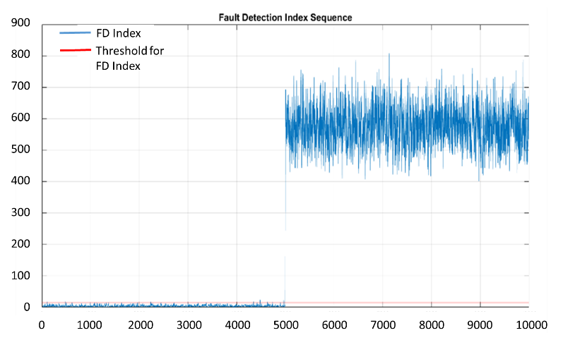Figure 10. Detection of two simultaneous faults

        Contribution analysis is similarly conducted in this case, where and . The associated results are illustrated in Figure 11. In this figure, since Sensor 1 and Sensor 2 have contributed the most to the violation of the fault detection index, it may be concluded that these two sensors are faulty.

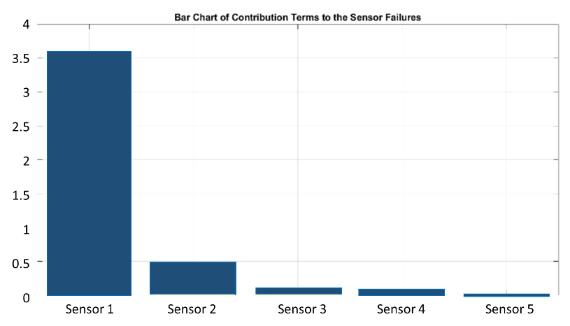                 Figure 11. Contribution analysis results of two simultaneous faults

7.       Conclusions

Combining analytic redundancy and contribution analysis, a novel methodology for fault detection, isolation, and reconstruction in MIMO dynamical systems has been proposed. It has been applied to a simulated jet engine control system. Numerical results have fully supported the correctness and effectiveness of the developed theory. Even for a slowly evolving incipient fault, the scheme can detect, isolate, and estimate it very effectively. Moreover, different sensor failures are also successfully detected and isolated, further justifying the practicability of the developed methodology.

One future research direction is the integration of our methodology to fault tolerant control systems and apply to power systems [10], aircraft [26], robots [27-28, 31], motors [11,32], planetary rovers [29], and missiles [33,34].

Conflict of Interest

The authors declare no conflict of interest.

1. R. Xu, C. Kwan, “Robust isolation of sensor failures” Asian Journal of Control, 5 (1), 12-23, March 2003. https://doi.org/10.1111/j.1934-6093.2003.tb00093.x
2. C. Kwan, R. Xu, “A note on simultaneous isolation of sensor and actuator faults” IEEE Trans. Control System Technology, 12 (1), 183-192, 2004. https://doi.org/ 10.1109/TCST.2003.821960
3. C. Kwan, R. Xu, W. Li, “A New Approach to Sensor Validation” in 21st Power Engineering Symposium, Taipei, Taiwan, 2000.
4. R. Xu, G. Zhang, X. Zhang, C. Kwan, K. Semega, “Sensor Validation Using Nonlinear Minor Component Analysis” in Third International Symposium on Neural Networks, Lecture Notes in Computer Science, Vol. 3973, 352-357, 2006. https://doi.org/10.1007/11760191_52
5. J. Cao, C. Kwan, R. Xu, F. Figueroa, “Simultaneous Sensor and Process Fault Diagnostics for Propellant Feed System” in 6th IFAC Symposium on Fault Detection, Supervision and Safety of Technical Processes, 2006.
6. X. Zhang, R. Xu, C. Kwan, M. Pritchard, L. Haynes, M. Polycarpou, Y. Yang, “Fault Tolerant Formation Flight Control of UAVs” Int. J of Vehicle Autonomous Systems, 2 (3/4), 217-235, 2004. https://doi.org/10.1504/IJVAS.2004.006108
7. M. Polycarpou, X. Zhang, R. Xu, Y. Yang, C. Kwan, “A Neural Network Based Approach to Adaptive Fault Tolerant Flight Control” in Proc. IEEE Int. Symposium on Intelligent Control, pp. 61-66, 2004. https://doi.org/10.1109/ISIC.2004.1387659
8. X. Zhang, M. M. Polycarpou, R. Xu, C. Kwan, “Actuator Fault Diagnosis and Accommodation for Improved Flight Safety” in Joint IEEE International Symposium on Intelligent Control and Mediterranean Conference on Control and Automation conference, pp. 640-645, 2005. https://doi.org/10.1109/.2005.1467089
9. X. Zhang, Y. Liu, R. Rysdyk, C. Kwan, R. Xu, “An Intelligent Hierarchical Approach to Actuator Fault Diagnosis and Accommodation” in IEEE Aerospace Conference, 2006. https://doi.org/10.1109/AERO.2006.1656088
10. J. Zhou, B. Ayhan, C. Kwan, S. Liang, W. Lee, “High performance arcing fault location in distribution networks” IEEE Trans. Industry Applications, 48 (3), 1107-1114, 2012. https://doi.org/10.1109/TIA.2012.2190819
11. C. Kwan, T. Qian, Z. Ren, H. Chen, R. Xu, W.-J. Lee, H. Zhang, J. Sheeley, “A Novel Approach to Corona Monitoring” Advances in Neural Networks – ISNN 2005: Second International Symposium on Neural Networks, Lecture Notes in Computer Science Volume 3498, pp 494-500, 2005. https://doi.org/10.1007/11427469_80
12. J. Qin, W. Li, “Detection, Identification and Reconstruction of Faulty Sensors with Maximized Sensitivity” AIChE J., 45 (9), 1963 – 1976, 1999. https://doi.org/10.1002/aic.690450913
13. A. Deluca, R. Mattone, “Actuator Failure Detection and Isolation Using Generalized Momenta” in IEEE Conference on Robotics and Automation, pp. 634– 639, September 2003. https://doi.org/10.1109/ROBOT.2003.1241665
14. X. Zhang, D. Miller, R. Xu, C. Kwan, H. Chen, “A Maximum Entropy based Approach to Fault Diagnosis Using Discrete and Continuous Variables” in 6th IFAC Symposium on Fault Detection, Supervision and Safety of Technical Processes, Beijing, 2006. https://doi.org/10.3182/20060829-4-CN-2909.00072
15. R. Xu, T. Qian, C. Kwan, “An Improved Optimal Pairwise Coupling Classifier” in International Symposium Neural Network, Advances in Neural Networks – ISNN 2005, Lecture Notes in Computer Science Volume 3497, pp 32-38 2005. https://doi.org/10.1007/11427445_6
16. P. Frank, “Fault diagnosis in dynamic systems using analytical and knowledge-based redundancy: A survey and some new results” Automatica, 26 (3), 459-474, 1990. https://doi.org/10.1016/0005-1098(90)90018-D
17. P. Nomikos, J. MacGregor, “Multivariate SPC charts for monitoring batch processes” Technometrics, 37 (1), 41-59, 1995. https://doi.org/10.2307/1269152
18. P. Miller, R. E. Swanson, C. E. Heckler, “Contribution plots: a missing link in multivariate quality control” Applied Mathematics and Computer Science, 8 (4), 775-792, 1998.
19. W. Li, S. Shah, “Structured residual vector based approach to sensor fault detection and isolation” J. of Process Control, 12 (3), 429-443, 2002. https://doi.org/10.1016/S0959-1524(01)00046-4
20. W. Li, C. Kwan, “A novel approach to sensor and actuator integrity monitoring” in IEEE Conference on Decision and Control, pp. 2140 – 2145, December 2016. https://doi.org/10.1109/CDC.2016.7798580
21. P. Van Overschee, B. de Moor, “N4SID: Subspace algorithms for the identification of combined deterministic-stochastic systems” 30 (1), 175-93, 1994. https://doi.org/10.1016/0005-1098(94)90230-5
22. R. Johnson, D. Wichern, Applied Multivariate Statistical Analysis, Prentice Hall, 5th Edition, 2001.
23. Z. Han, W. Li, S. Shah, “Fault detection and isolation in the presence of process uncertainties” Control Engineering Practice, 13 (5), 587-599, 2005. https://doi.org/10.1016/j.conengprac.2004.04.020
24. P. Geladi, B. Kowalski, “Partial least-squares regression: A tutorial” Analytica Chimica Acta, 185 (1), 1-17, 1986. https://doi.org/10.1016/0003-2670(86)80028-9
25. R. J. Patton, J. Chen, “Robust fault detection of jet engine sensor systems using eigenstructure assignment” J. of Guidance, Control, and Dynamics, 15 (6), 1491-1497, 1992. https://doi.org/10.2514/3.11413
26. M. Ciuryla, Y. Liu, J. Farnsworth, C. Kwan, M. Amitay, “Flight Control Using Synthetic Jets on a Cessna 182 Model,” Journal of Aircraft, 44(2), 642-653, 2007. https://doi.org/10.2514/1.24961
27. C. Kwan, K. S. Yeung, “Robust Adaptive Control of Revolute Flexible-Joint Manipulators Using Sliding Techniques,” Systems and Control Letters, 20(4), 279-288, 1993. https://doi.org/10.1016/0167-6911(93)90004-P
28. C. Kwan, “Robust Adaptive Force/Motion Control of Constrained Robots,” IEE Proceedings Pt. D, 143(1), 103-109, 1996. https://doi.org/10.1049/ip-cta:19960090
29. B. Ayhan, M. Dao, C. Kwan, H. Chen, J. F. Bell III, R. Kidd, “A Novel Utilization of Image Registration Techniques to Process Mastcam Images in Mars Rover with Applications to Image Fusion, Pixel Clustering, and Anomaly Detection,” IEEE Journal of Selected Topics in Applied Earth Observations and Remote Sensing, 2017. https://doi.org/10.1109/JSTARS.2017.2716923
30. Kronecker product, http://www.math.uwaterloo.ca/~hwolkowi/henry/reports/kronthesisschaecke04.pdf
31. C. Kwan, F. L. Lewis, Y. H. Kim, “Robust Neural Network Control of Flexible-Joint Robots,” Asian Journal of Control, pp. 188-197, vol. 1, no.3, September, 1999. https://doi.org/10.1111/j.1934-6093.1999.tb00019.x
32. P. Ballal, A. Ramani, M. Middleton, C. McMurrough, A. Athamneh, W. J. Lee, C. Kwan, F. L. Lewis, “Mechanical Fault Diagnosis using Wireless Sensor Networks and a Two-Stage Neural Network Classifier,” Proc. IEEE Aerospace Conference, 2009.https://doi.org/10.1109/AERO.2009.4839671
33. C. Kwan, R. Xu, W. Liu, R. Tan, L. Haynes, “Nonlinear Control of Missile Dynamics,” in Proc. IEEE Conference on Decision and Control, pp.4685-4691, 1998. https://doi.org/10.1109/CDC.1998.762073
34. D. Li, J. B. Cruz, Jr., G. Chen, C. Kwan, H. Chang, “A Hierarchical Approach to Multi-Player Pursuit-Evasion Differential Games,” in 44th IEEE Conference: Decision and Control, 2005 and 2005 European Control Conference, pp. 5674-5679, 2005. https://doi.org/10.1109/CDC.2005.1583067

(Click to view)

(Click to view)