A Comparison of Mean Models and Clustering Techniques for Vertebra Detection and Region Separation from C-Spine X-Rays

Adv. Sci. Technol. Eng. Syst. J. 2(3), 1758–1770 (2017);
 DOI: 10.25046/aj0203215
In Computer Aided Diagnosis (CAD) tools, vertebra localization and detection are the essential steps for the diagnosis of cervical spine injuries. The accurate localization leads to accurate treatment, which is more challenging in case of poor contrast and noisy radiographs. This paper targets c-spine radiographs for the localization of vertebra using different vertebra templates, vertebra detection at each level using two different clustering techniques and gives a comparison between them. Moreover it separates the regions for each individual c-spine. It takes the poor contrast x-ray as input, enhance the contrast and detect the edges of enhanced image. After the edge detection, manually selected Region of Interest (ROI) helps in getting the edges of area covering C3 – C7 only. These edges along with 4 different template models of vertebra are used for the localization by Generalized Hough Transform (GHT). The results obtained are analyzed visually for the best localization template. Then, on voted points obtained after pruning, two clustering techniques Fuzzy C Means and K-Means are applied separately, to form clusters and centroids for each vertebra. Another part of this paper is to separate vertebra regions. For this, intervertebral points are calculated and then along these points, centroids are rotated using Affine Transformation. It gives parallel lines to vertebrae and joining them gives region for each vertebra. The comparison and testing of proposed technique has been performed using dataset ‘NHANES II’ publicly accessible at ‘The National Library of Medicine’, total 150 cervical spine scans are used securing accuracies 93:76%, 84:21% and 83:1% for FCM, K-Means and region separation, respectively.
1. Introduction
Spinal cord proves to be the most important element of human anatomy. It works as a backing for other segments of human body so that one can bend, twist and move easily. If this most essential segment of human structure is damaged in any way, a person cannot even stand up straight. Figure 1 illustrates the division of human spinal cord which consists of 33 individual bones known as vertebra. First 7 cervical vertebra (C1 ? C7) collectively form the neck, next 12 thoracic vertebra (T1 ? T12) form the chest, next 5 lumbar vertebra (L1 ? L5) form the lower back, next 4 sacral vertebra (S1 ? S4) form the pelvis and the last 4 fused vertebra form the tail bone of human structure are known as coccyx bones.
In the past few decades, medical imaging has been segments of human body so that one can bend, twist developed in dramatic way and helping radiologists and move easily. If this most essential segment of hu- for the diagnosis and treatment of cervical spine disman structure is damaged in any way, a person can- orders including osteoporosis, cervical spine injuries not even stand up straight. Figure 1 illustrates the and trauma [3]. The most common sources for cdivision of human spinal cord which consists of 33 spine injuries (CSI) are accident of vehicles and outindividual bones known as vertebra. First 7 cervi- door games and fall down [1][2]. In youngsters age cal vertebra (C1 − C7) collectively form the neck, next ranging 15-25, hyperextension and vehicles accident 12 thoracic vertebra (T1 − T12) form the chest, next 5 where as in senior citizens and osteoarthritic victims, lumbar vertebra (L1 − L5) form the lower back, next 4 sudden fall is reported as the most common reason of CSI [4]. Latterly, a significant amount of Traumatic Spinal Cord Injuries (TSCI) has been reported which may become more problematic and critical if the patient is not treated on time by accurate diagnosis [5].
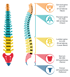 Figure 1: Spinal Column: Anatomical Features
In Computer Aided diagnosis (CAD) tools, vertebra localization and detection at each cervical level are initial and essential steps to be performed and it becomes more difficult when images are low contrast and noisy like X-rays. These steps work significantly in many orthopedics and neurological applications for the diagnosis and treatment of spinal column disorders. The accurate localization and detection leads to accurate treatment of abnormalities. Thus, great success rate in vertebra localization and detection with separated regions for each vertebra would be very helpful for radiologists’ community, not only for the diagnosis but also in surgeries. Figure 2 shows the (a) Normal cervical spine x-ray with perfect relationship between posterior, anterior and spinolaminar lines. They are aligned representing a healthy radiograph where as (b) shows loss of alignment at C6 and C7 representing unhealthy or fractured X-ray.
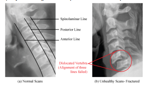 Figure 2: C-Spine Radiographs (a) Healthy (b) Fractured
This figure shows that the fractures can be located using parameters like posterior, anterior and spinolaminar lines by getting the alignment information between them. In literature, many techniques like Generalized Hough Transform (GHT) [6], Active Shape Model (ASM) [7], discrete dynamic contour model (DDCM) [8] and Template Matching [9] have been described for the localization, detection and segmentation of spinal cord using different set of images including magnetic resonance imaging (MRI) and computed tomography (CT) scans. Klinder et al. [10] described a methodology for the extraction of vertebra shape using CT scans. They designed a methodology for the detection, identification and segmentation of vertebra from CT scans. They applied Generalized Hough Transform (GHT) with the combination of adapted triangulation shape for the localization and segmentation of vertebra. They tested the proposed technology on 64 CT Scans with success rate of 70%. Alomari et al. [11] presented a methodology of localization using MRI images. They used two datasets of 50 and 55 scans attaining success rate of 87% and 89.1%. Their proposed model was based on two steps targeting intervertebral discs. Korez et al. [12] presented an automated technique for the detection and segmentation of vertebra and spine using 3D CT Scans. They used interpolation theory for the localization of spine which is further used to locate the individual vertebra. The localization results obtained helped in the segmentation of each vertebra by enhanced shape-constrained deformable model approach. They tested the technique using two CT Scans databases of 50 lumbar and 170 thoracolumbar vertebrae and achieved high success rate. Lecron et al. [13] presented a methodology taking benefit of edge polygonal approximation to locate the vertebra and perform the segmentation using Active Shape Model (ASM). They enhanced the performance of the methodology by parallel computing and heterogeneous architectures for the vertebra extraction. They used X-ray images for the testing of proposed methodology. Larhmam et al. [14] described a technique for the vertebra localization targeting x-rays image. They used a novel combination of GHT and Kmeans clustering for the localization of vertebra using template matching theory. Benjelloun et al.[15] presented an analysis of vertebra based on segmentation from x-ray images. They described a relative study of two algorithms to segment out vertebra. Lecron et al. [16] presented a model targeting the vertebra localization from X-rays using SVM model and SIFT descriptor. They evaluated their methodology using 50 scans and attained satisfactory success rate of 81.6%. Dong et al. [17] presented a graphical model based vertebra identification which need no training steps for processing. They designed it to automatically detect the total number of visible vertebra in scans and localize them. Larhman et al. [18] described a localization technique by offline training of template model as a preprocessing step and applied GHT to localize the vertebra. Then they performed the post processing of model using adaptive filter and attained success rate of 89% when tested by 200 vertebrae. Benjelloun et al. [19] proposed a scheme based on polygon regions for the extraction of vertebra boundries and perform segmentation. Later in [20], they presented a technique for the localization and segmentation based on ASM.
This paper is basically an extension of model originally presented in IEEE International Conference on Communication, Computing and Digital Systems (CCODE 17)[21]. This paper is extended in terms of comparison of template models for better localization and then a comparison and analysis of clustering techniques used for the detection of centroids. A section which is extension to original paper, is dedicated to the region separation for each individual vertebra which can be used further for the segmentation process and will be very helpful for the diagnosis of several c-spine disorders. Section II describes the methodology of proposed technique, Results are analyzed and discussed in Section III and Section IV presents the conclusion of this paper.
2. Methodology
The presented technique comprises five stages to give a comparison of techniques for better localization and detection results along with separated regions for each vertebra. The flow chart of presented model is shown in Figure 4, representing the main steps of model including Preprocessing, Creation of Mean models, Vertebra Localization, Centroid detection and Region separation.
2.1. Preprocessing
Preprocessing is the first and most significant stage of the presented model for attaining high success rate. The steps involved in this stage are contrast enhancement, detection of edges and manual selection of Region of Interest (ROI). These steps are performed to get enough data for our vertebra localization stage.
2.1.1. Contrast enhancement
The input X-ray images are poor contrast and noisy set of images which cannot be processed directly to achieve high accuracy of presented technique. The superimposition of other bony structures and level of brightness at C6 and C7 leads to wrong localization results. So ‘Contrast Limit Adaptive Histogram Equalization’(CLAHE) [22] is applied to input radiographs so that the contrast can be enhanced for better results. CLAHE works like ordinary adaptive histogram equalization, the only difference is it uses a specific threshold to clip the histogram. For X-ray images, CLAHE is one of the most efficient contrast enhancement algorithm when compared with Gamma Correction (GC) and Histogram Equalizer (HE)[23].
2.1.2. Detection of edges
After the contrast enhancement, the edges of input image are detected using ‘Canny Edge Detector’ [24]. The reason behind the edge detection is that the GHT algorithm works with edges only. The process of localization takes place using edges. So we detected the edges of input image for any further processing.
2.1.3. Manual selection of Region of Interest (ROI)
The edge detection step gives us the edges of whole input image, but the proposed technique requires edges for the C3−C7 only. so in this step we constructed the Region of Interest (ROI) covering the area of lower 5 cervical vertebrae only. Then this ROI is multiplied with the edges to get the edges of this area only. This is the last step of our Preprocessing stage.
2.2. Creation of Mean Models
The creation of mean models is next stage of proposed technology. In this stage, 4 different template models M1, M2, M3 and M4 are constructed and shown in Figure 3. For the construction of these template models, 25 vertebra images for each template model are created using some drawing tools and then mean image is created using these 25 images. Eq. 1 is used to create mean model of each shape.
Vt
1 X
Mi = Vx (1)
Vt x=0
where ‘Vt’ presents the total vertebra images (25) created manually and ‘Vx’ is one vertebra image with ‘x’ varying from 1 to 25.
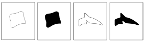 Figure 3: Vertebra Models created: (a) M1 (b) M2 (c)
M3 (d) M4
The reason behind using these 4 mean models is just to analyze the results and give a comparison between them. So that one can select best mean model for localization of vertebra securing high accuracy. M1 and M2 represents the body of vertebra whereas M3 and M4 represents complete vertebra shape including body. These created models will be used as a template image for the detection process of GHT. The results are generated using all four template images one by one and then analyzed visually to select the best template image.
2.3. Vertebra Localization(GHT)
The third and most important stage of proposed methodology is Vertebra Localization which helps in the detection of centroids. In this stage, the selected
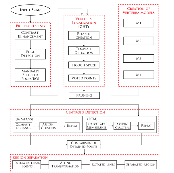 Figure 4: Flow Chart: Main stages of the proposed methodology
edges of Preprocessing stage are used and GHT is applied. Ab initio, Hough Transform [25] was introduced as a technique for the detection of lines, circles, elipse etc following a modified concept by Ballard, known as generalized Hough Transform [6] used in various applications of image processing and computer vision. GHT is a concept used widely for the detection of arbitrary shapes and pattern recognition in all fields of imaging including biomedical imaging. The most positive point of this technique is it is invariant to any kind of transformations. It works with two factors R-Table which basically represents the template model of vertebra which is to be detected in the image and second one is Accumulator, which is Hough Space and stores the voted points localizing the area of C3 − C7. GHT is based on the template matching theory and uses the information stored in R-Table for the detection process.
2.3.1. R-Table creation
For the construction of R-table, a reference point (rx,ry) is selected. The coordinates of extracted edges helped in this regard. The reference point is selected by taking the mean of all the edges and next, gradient is calculated. Then for each point, gradient direction is computed and saved as a function of gradient. There are more than one entries of gradient direction for each value of gradient. So, in R-table each entry is the difference between the coordinates of reference point and boundary point w.r.t the direction of gradient. In this way, the template model of vertebra is stored as a R-Table. Table 1 [6] represents the generic form of R-table, where Φ, dr and β represents gradient, distance and orientation, respectively. The distance and orientation are calculated using Eq. 2 and Eq. 3, respectively.
q
| dr = (rx −bx)2 +(ry −by)2 | (2) |
| b −
β = tan−1 y ry |
(3) |
bx −rx
where in both equations (rx,ry) is the reference point and (bx,by) is the boundary point.
| Orientation Φ | Position (r,β) |
| 0 | (rx,βx)/Φx = 0 |
| Φ | (rx,βx)/Φx = ∆Φ |
| 2∆Φ | (rx,βx)/Φx = 2∆Φ |
| 3∆Φ | (rx,βx)/Φx = 3∆Φ |
| … | … |
Table 1: R-Table: Generic Form
2.3.2. Template detection and Hough Space
Now, for the detection process an Accumulator is created which represents the Hough Space and stores the points known as Voted points. These points mark the positions containing the template model. So, for each edge point obtained in preprocessing stage, gradient is computed and the corresponding value of R-Table stored as r(Φ) is added into the coordinates of edge point. Then the model check the resultant value if it is within the scope of Accumulator, if yes it increments the location of accumulator defined by this new point. All the voted points obtained by this process give the positioning of vertebra in X-rays. However, few outliers are also calculated by this process which are removed in next step.
2.3.3. Pruning
Pruning [26] is a technique used to remove unwanted data points known as outliers. These outliers may effect the success rate of the proposed model. The window scheme is applied and voted points are removed if they are less than the specified number. Then the voted points obtained after pruning are used for the centroid detection. For each candidate point, a window placed such that candidate point lies at center of window and all points lying inside window are computed. Now, if the count of points is less than a specific number then that candidate point is removed.
2.4. Centroid Detection of vertebra body
After the localization of vertebra from C3−C7, the next stage of proposed technique is to detect the centroids of each vertebra using the voted points obtained by all four template models. The centroid detection is performed using two different clustering techniques K-Means and Fuzzy C Means. Each clustering technique forms clusters using the voted points and then gives the centroid for each cluster representing each vertebra (C3−C7).
2.4.1. K-Means clustering
K-Means [27] is a clustering algorithm works simply to segment out the data into clusters by calculating the euclidian distance between them. Initially, the cluster’s center are selected randomly from obtained voted points, it randomly selected the 5 cluster centers representing 5 cervical vertebra (C3 − C7). Then for each voted point, euclidean distance is calculated between the voted point and all the cluster centers. And the cluster at minimum distance is assigned to that voted point. This process is performed for all the voted points, completing the first iteration of k-means algorithm. For next iteration, cluster centers are selected by calculating the mean of all the points belonging to the same cluster. Then again distance computation is carried out and clusters are assigned and this process continues until two or more consecutive iterations give same results. The cluster centers obtained in last iteration represents the centroid of each vertebra.
2.4.2. Fuzzy C Means clustering
Fuzzy C-Means (FCM) is another clustering technique developed by Dunn [28] in 1973, then in 1981, Bezdek [29] enhanced the working of this algorithm. It works with the concept of fuzziness and assign clusters in such a way that one data point may belong to more than one cluster at a time. It assign membership to each data point for all the clusters. The range of membership varies from 0 to 1. This factor of fuzziness makes FCM less sensitive to outliers. Initially, FCM selected the 5 cluster centers randomly representing 5 cervical vertebra. Then for each voted point, total 5 memberships are computed, between this point and all the cluster centers. The membership varies from 0 to 1 and is computed using Eq. 4 which basically gives the information about the point that how much this point relates to which cluster. The cluster with greatest membership is the most closes to that voted point.
1
mjx =(4)
kbj−cxk t
i=1 kbj−cik
where ‘i’ varies from 1 to ‘t’ representing the total clusters i-e 5, ‘cx’ and ‘bj’ represents the cluster and voted point for which membership is to be calculated, respectively. This process of assigning memberships creates a level of fuzziness and one voted point belongs to more than one cluster at a time. First iteration is completed, after calculating the membership for all the voted points and new cluster centroids are selected using Eq. 5
tp j
P m .p i=1 ix j
cx = Ptp j (5) m
i=1 ix
where ‘cx’ and ‘tp’ represents the new cluster computed and total number voted points, respectively. Then in next iteration for these new computed cluster centroids, membership is calculated and this process continues until we get similar centroids in 2 or more consecutive iterations, representing the 5 cervical vertebra from C3 to C7.
2.5. Separation of vertebra regions
The separation of each vertebra region is another stage and extension to original work, which allows us to extract the region for vertebra individually using the center points of vertebra. These extracted regions are very helpful in the segmentation process which further leads to the diagnosis of many spinal cord disorders. The steps involved in this stage are calculation of Intervertebral Points and Affine Transformation.
2.5.1. Intervertebral Points
To extract the regions covering the area for each vertebra,intervertebral points are required. The intervertebral points are the location between the two vertebra. In our case we required total 6 intervertebral points, from which 4 are easy to find out by just calculating the mean of centroids from C3− C7 which we already have. Eq.6 represents the calculation of these 4 intervertebral points.
IVCi = (Ci +Ci+1)/2 where i = 3,4,5,6 (6)
The other two intervertebral points, one before C3 and second after C7 couldn’t be computed using this equation as it require centroids before and after these points. So, a simple technique using equations 7 and 8 is applied to obtained these two intervertebral points. The difference between C3 and IVC3 is subtracted from the coordinates of C3 to get an estimated intervertebral point before C3 i-e IVC2
IVC2 = C3−(IVC3 −C3) (7)
Similar technique using C7 and IVC6 is applied for IVC7 but instead of subtracting the difference, it is added into the coordinates of C7 to get points greater than it’s location.
IVC7 = C7 +(C7−IVC6) (8)
Now, for next step there are total 11 points, 6 intervertebral and 5 centroids in the same sequence as IVC2, C3, IVC3,…,C7, IVC7.
2.5.2. Affine Transformation
A transformation following the rule of collinearity is known as Affine Transformation [30]. The term collinearity defines that points stay on a line at same distance and the parallel lines remains parallel, before and after the transformation. But in case of parallel lines, collinearity is not applicable on the angles between them. The term Affine Transformation is also called Affinity.
In proposed technique, affine transformation is used to form lines parallel to the vertebra. For each line, 3 points of vertebra are required, and location of two points is transformed in such a way that they stay on same line before and after the transformation, Affine Map helps in this regard. The calculation of Affine Map is shown in Eq. 9 where ‘a’, ‘R’ and ‘c’ are rotational point, rotational matrix and directional matrix, respectively. These three matrices are the general Affine transformation matrix.
M = a∗R∗c (9)
The rotational matrix requires angle Θ to rotate the lines accurate enough and make them parallel to each vertebra. To obtain this angle, initially two angles are calculated: one between the first intervertebral point and centroid and second between the centroid and next intervertebral point, then taking average of these two angles and adding 90 into it, gives an exact angle for making lines parallel. Using this angle Θ +90, Affine Map is constructed using Eq. 9 and multiplied with each point to rotate them along intervertebral points. As a result, total 6 lines are formed covering C3 to C7. Then these lines are joined to make separate regions for each vertebra.
3. Results and Evaluation of proposed technique
The proposed technique has been implemented in MATLAB R2013a. The dataset NHANES II [31] used for the evaluation of our proposed technique is publicly accessible at U.S. National Library of Medicine, incorporating 17,000 scans (10,000 cervical spine and 7,000 lumbar) of patients age ranging 25-74, captured in 1976-1980. These X-rays images had been taken under varying scale, orientation and environment. For evaluation of our proposed technique we used 150 cervical spine scans of this dataset, selected on random basis. In literature, several methods has been tested using the same dataset but varying number of images. In these papers, no one ever mentioned the criteria following which they has selected the specific number of images. Neither they defined exactly which images has been selected. So it is clear that everyone is using different images of the same dataset. For fair testing, we selected subset with larger number of images than literature. For the comparison of results, a ground truth is maintained by visually examining each image. For each image, 5 center points representing each vertebra body are marked manually, targeting C3 to C7. These annotated points are stored and used for the testing purposes. A comparison of FCM and K-Means is given in this section using Statistical and Visual results.
3.1. Statistical Results
The parameters used to obtain the statistical results include pixel distance, mean, standard deviation and accuracy.
3.1.1. Pixel distance
Figure 8 shows the pixel distance of 50 images for both K-means and FCM. For better visualization, the result of 50 images is shown in figure but is calculated for all 150 images. Each graph represents each vertebra with red dotted line representing the mean distance of K-means and black dotted line is for FCM, for all 150 images. The difference is calculated between the annotated points and detected centroids, representing how much detected centroid is away from the center point. The mean error lines show that at each vertebra level FCM works better than K-Means, the mean error for FCM is less than that of K-Means, but at level C7 there is a minor difference between the two. The presence of high brightness and superimposition of other structures make the false detection at this cervical level.
3.1.2. Mean
Figure 5 shows the calculated mean of the distance. The green bar shows the mean of k-means which is larger than FCM at every level, represented by blue bar. This parameter also marked FCM as a better
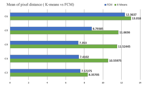 Figure 5: Mean of calculated distance: K-Means vs
FCM
clustering technique for centroid detection of vertebra from X-rays. The eq. 10 is used for the calculation of mean.
PTi=1di (10)
Meanerror = T
Where ‘di’ represents the distance at each cervical and ‘T’ represents total images used.
3.1.3. Standard Deviation
The standard deviation is another statistical parameter of our presented methodology. Figure 6 shows the calculated standard deviation in both cases.
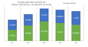 Figure 6: Standard Deviation: K-Means vs FCM Each level shows less variation in case of FCM than K-means, making FCM better than the K-Means. The standard deviation is calculated using Eq. 11
sPT (di −Meanerror)2
SD = i=1 (11) T −1
where ‘di’, ‘Meanerror’ and ‘T ’ represents distance, calculated mean and total number of images, respectively.
3.1.4. Accuracy
The accuracy of presented technique is measured at two levels Visual and Experimental. In case of visual accuracy, labels are assigned to all 150 images at each cervical label.
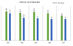 Figure 7: Visual accuracies reported at each cervical level
If the detected vertebra is correct label ‘1’ is assigned and in case of wrong detection label ‘0’ is assigned. The presented model consider the vertebra detection as correct if it is within the body of vertebra.So in visual examination, this point is followed for labeling process and each vertebra has been given label ‘1’ if it is inside or on the boundary of vertebra body and ‘0’ is it is outside the vertebra body. Using this criteria all the images has been assigned total 5 labels representing 5 vertebra and then using these labels overall accuracy of 94.7% and 79.4% are measured for FCM and K-Means, respectively.
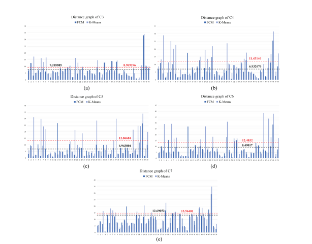 Figure 8: Pixel wise Distance Graph: (a)C3 (b)C4 (c)C5 (d)C6 (e)C7 Figure 8: Pixel wise Distance Graph: (a)C3 (b)C4 (c)C5 (d)C6 (e)C7 |
The accuracies at each cervical level are shown in figure 7 where green bars are representing greater accuracies for FCM than the K-means represented by blue bars.
Similar method of labeling is used for measuring the accuracies of separated regions. An overall accuracy of 83.1% is reported for separated regions with 90.5%, 93%, 88.5%, 73%, 70.5% at each cervical level from C3 to C7, respectively. In case of Experimental accuracies, ROC curves are formed for both FCM and K-Means shown in figure 9. Each line represents the accuracy measure of each cervical level from C3 to C7 with varying threshold from 0 to 20. The threshold here represents the width of vertebra. We selected threshold 14 for the accuracies, the reason behind choosing threshold 14 is, it is the radius of vertebra which means all the point inside the vertebra body are correctly detected. At threshold 14 the proposed technique attained accuracy of [93.12, 85.79, 81.30, 81.52, 79.30]and [96.74, 96.65, 95.51, 95.33, 84.55] representing C3, C4, C5, C6 C7 for K-Means and FCM, respectively.In both cases, visual and experimental accuracies FCM secured more accuracy than k-means.
The accuracy when compared with other techniques in literature, it has been observed that only Larhman [14] secured greater accuracy of 97.5% than proposed technique i-e 93.6%. But it is not a fair comparison as both are using different subset of same dataset. They used 66 images of NHANES II dataset whereas presented methodology has been tested using 150 images of NHANES II dataset.
3.2. Visual Results
The visual analysis of each stage are shown in this section including steps of each stage. All the results shown are of 5 different cases of NHANES II dataset. Each column represents different case, whereas each row represents each step.
3.2.1. Preprocessing
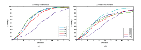 Figure 9: Receiver Operating Characteristic (ROC): (a) FCM Clustering (b) K-Means Clustering Figure 9: Receiver Operating Characteristic (ROC): (a) FCM Clustering (b) K-Means Clustering |
Figure 10 shows the visual results of first stage i-e Preprocessing of proposed technology. The first row shows the low contrast input x-rays which are enhanced by using CLAHE and shown in second row, it is clearly observed that the contrast of second row is improved and now these images can be used for better results. Next row shows the result of edge detection step, the edges are extracted for complete input image which are reduced to the ROI C3 − C7 and shown in 4th row.
3.2.2. Creation and selection of vertebra Models
The next stage of our model is creation of different vertebra models and figure 11 shows the results obtained by these models. Each row shows the detected centroids obtained using different models but same cases and it is clearly observed that M1 has given the most accurate results than other models.
3.2.3. Vertebra Localization (GHT)
The visual results obtained in vertebra localization stage are shown in figure 12, first row represents the hough space created by each case and voted points are represented in row 2, row 3 shows the voted points obtained after pruning where many outliers are removed, which can be observe in row 2.
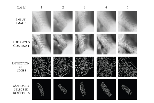 Figure 10: Phase 1: Preprocessing
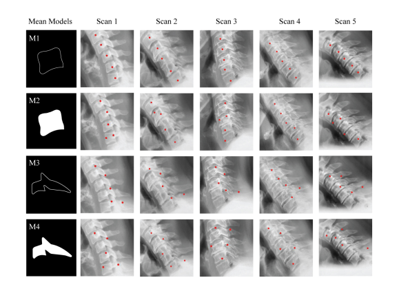 Figure 11: Phase 2: Comparison of different vertebra models
3.2.4. Centroid Detection
The centroid detection is carried out using two clustering techniques and their results are shown in figure 13 where first two rows represent the clusters and next two rows represents the detected centroids for each vertebra using K-Means and FCM clustering, respectively. Last row represents a comparison between annotated centroids (blue points), FCM centroids (red points) and K-Means (magenta point). It is clearly observed that FCM works way much better than the KMeans. In same cases FCM marked the correct centroids where as K-Means failed to do so.
3.2.5. Separation of vertebra regions
The steps involved in the separation of vertebra regions are shown in figure 14 where first row shows the blue centroids and 4 intervertebral points marked by red star. In next row, two additional intervertebral points are shown by yellow stars. The rotated lines by Affine transformation can be observed in 3rd row. Then after joining lines the separated regions are shown in 4th column.
4. Conclusion
This paper presents a comparison between 4 different vertebra template models for localization and 2 clustering techniques for centroid detection of cervical vertebra from x-ray images. The proposed model gives the separated regions for 5 targeted vertebra C3 − C7. The comparison of clustering techniques, vertebra template models and region separation technique is the contribution to this paper. For the localization of vertebra, GHT is applied along with each template model and results are analyzed. For GHT, M1 proves to be the best vertebra template. The voted points obtained after pruning are used for centroid detection. For the detection procedure two different clustering techniques are used FCM and K-Means. The results obtained by these two clustering techniques are analyzed at statistical and visual level and FCM proves to be much better than K-Means clustering for the detection of c-spine from x-rays. The results at level C7 are less than the other levels in both clustering techniques, reason behind this is the presence of high brightness and other structures which are superimposed. The testing and comparison of proposed technique has been performed using 150 scans of NHANES II dataset accessible publically at U.S National Library of Medicine. The obtained accuracies of centroid detection are 84.21 and 93.76 for K-means and FCM, respectively. From all the experiments it is concluded that the FCM is more accurate than the K-means for the localization and detection of cervical verterba from X-rays. It is due to the fact that the fuzziness of FCM makes it less sensitive to outliers
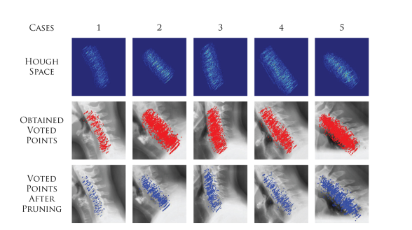 Figure 12: Phase 3: Visual results of vertebra localization steps
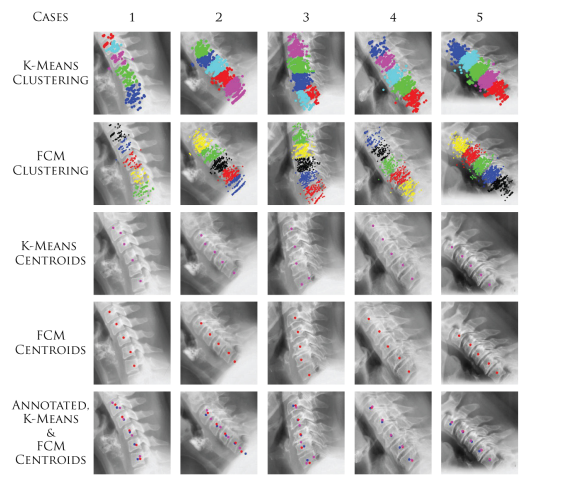 Figure 13: Phase 4: Centroid detection and comparison of clustering techniques
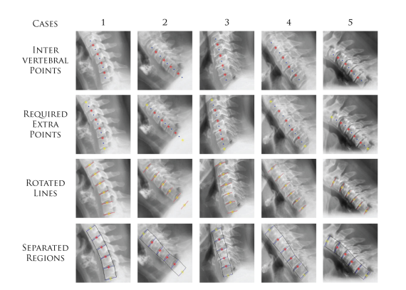 Figure 14: Phase 5: separation of vertebra regions
than K-means. Moreover, the proposed method secured satisfactory success rate of 83.1% for the separated regions which can be increased by increasing the width of the parallel lines. In future, our work is focused on segmentation using the separated regions and detected centroids.
- R. M. Hasler, A. K. Exadaktylos, O. Bouamra, L. M. Benneker, M. Clancy, R. Sieber, H. Zimmermann, and F. Lecky, “Epidemiology and predictors of cervical spine injury in adult major trauma patients: a multicenter cohort study,” Journal of trauma and acute care surgery, vol. 72, no. 4, pp. 975–981, 2012.
- J. W. Tee, P. C. Chan, R. L. Gruen, M. C. Fitzgerald, S. M. Liew, P. A. Cameron, and J. V. Rosenfeld, “Early predictors of mortality after spine trauma: a level 1 Australian trauma center study,” Spine, vol. 38, no. 2, pp. 169–177, 2013.
- L. A. Nadalo, “Thoracic Spinal Trauma Imaging,” Accessed on: April 06, 2016.
- P. J. Richards, “Cervical spine clearance: a review,” Injury, vol. 36, no. 2, pp. 248–269, 2005.
- V. Rahimi-Movaghar, M. K. Sayyah, H. Akbari, R. Khorramirouz, M. R. Rasouli, M. Moradi Lakeh, F. Shokraneh, and A. R. Vaccaro, “Epidemiology of traumatic spinal cord injury in developing countries: a systematic review,” Neuroepidemiology, vol. 41, no. 2, pp. 65–85, 2013.
- D. H. Ballard, “Generalizing the hough transform to detect arbitrary shapes,” Pattern Recognition, vol. 13, no. 2, pp. 183– 194, 1991.
- T. F. Cootes, C. J. Taylor, et al., “Statistical models of appearance for computer vision,” 2004.
- S. Lobregt and M. A. Viergever, “A discrete dynamic contour model,” IEEE transactions on medical imaging, vol. 14, no. 1, pp. 12–24, 1995.
- R. Brunelli, Front Matter. Wiley Online Library, 2009.
- T. Klinder, J. Ostermann, M. Ehm, A. Franz, R. Kneser, and C. Lorenz, “Automated model-based vertebra detection, identification, and segmentation in {CT} images,” Medical Image Analysis, vol. 13, no. 3, pp. 471 – 482, 2009.
- A. Raja’S, J. J. Corso, and V. Chaudhary, “Labeling of lumbar discs using both pixel-and object-level features with a two level probabilistic model,” IEEE transactions on medical imaging, vol. 30, no. 1, pp. 1–10, 2011.
- R. Korez, B. Ibragimov, B. Likar, F. Pernus, and T. Vrtovec, “A framework for automated spine and vertebrae interpolationbased detection and model-based segmentation,” IEEE transactions on medical imaging, vol. 34, no. 8, pp. 1649–1662, 2015.
- F. Lecron, S. A. Mahmoudi, M. Benjelloun, S. Mahmoudi, and P. Manneback, “Heterogeneous computing for vertebra detection and segmentation in x-ray images,” Journal of Biomedical Imaging, vol. 2011, p. 5, 2011.
- M. A. Larhmam, M. Benjelloun, and S. Mahmoudi, “Vertebra identification using template matching modelmp and kmeans clustering,” International journal of computer assisted radiology and surgery, vol. 9, no. 2, pp. 177–187, 2014.
- M. Benjelloun and S. Mahmoudi, “X-ray image segmentation for vertebral mobility analysis,” International journal of computer assisted radiology and surgery, vol. 2, no. 6, pp. 371–383, 2008.
- F. Lecron, M. Benjelloun, and S. Mahmoudi, “Fully automatic vertebra detection in x-ray images based on multi-class svm,” in SPIE Medical Imaging, pp. 83142D–83142D, International Society for Optics and Photonics, 2012.
- X. Dong and G. Zheng, “Automated vertebra identification from x-ray images,” Image Analysis and Recognition, pp. 1–9, 2010.
- M. A. Larhmam, S. Mahmoudi, and M. Benjelloun, “Semiautomatic detection of cervical vertebrae in x-ray images using generalized hough transform,” in Image Processing Theory, Tools and Applications (IPTA), 2012 3rd International Conference on, pp. 396–401, IEEE, 2012.
- M. Benjelloun and S. Mahmoudi, “Spine localization in x-ray images using interest point detection,” Journal of digital imaging, vol. 22, no. 3, pp. 309–318, 2009.
- M. Benjelloun, S. Mahmoudi, and F. Lecron, “A framework of vertebra segmentation using the active shape model-based approach,” Journal of Biomedical Imaging, vol. 2011, p. 9, 2011.
- A. Mehmood, M. U. Akram, and A. Tariq, “Vertebra localization and centroid detection from cervical radiographs,” in Communication, Computing and Digital Systems (C-CODE), International Conference on, pp. 287–292, IEEE, 2017.
- K. Zuiderveld, “Contrast limited adaptive histogram equalization,” in Graphics gems IV, pp. 474–485, Academic Press Professional, Inc., 1994.
- I. A. M. Ikhsan, A. Hussain, M. A. Zulkifley, N. M. Tahir, and A. Mustapha, “An analysis of x-ray image enhancement methods for vertebral bone segmentation,” in Signal Processing & its Applications (CSPA), 2014 IEEE 10th International Colloquium on, pp. 208–211, IEEE, 2014.
- P. Zhou, W. Ye, Y. Xia, and Q. Wang, “An improved canny algorithm for edge detection,” Journal of Computational Information Systems, vol. 7, no. 5, pp. 1516–1523, 2011.
- R. O. Duda and P. E. Hart, “Use of the hough transformation to detect lines and curves in pictures,” Commun. ACM, vol. 15, pp. 11–15, Jan. 1972.
- E. R. Dougherty and R. A. Lotufo, Hands-on morphological image processing, vol. 59. SPIE press, 2003.
- K. Alsabti, S. Ranka, and V. Singh, “An efficient k-means clustering algorithm,” 1997.
- J. C. Dunn, “A fuzzy relative of the isodata process and its use in detecting compact well-separated clusters,” 1973.
- P. Wang, “Pattern-recognition with fuzzy objective function algorithms-bezdek, jc,” 1983.
- C. C. Stearns and K. Kannappan, “Method for 2-d affine transformation of images,” Dec. 12 1995. US Patent 5,475,803.
- “NHANES II X-ray Images,” Jan 27,2016