1. Introduction

1.1    Topic of the work

This paper is an extension of [1]. The topic of this work is application of Conformal Prediction (CP) framework of reliable machine learning to big data. Conformal Prediction was developed in such works as [2, 3]. Its main advantage is producing prediction sets that are valid in weak (i.i.d./exchangeability) as-sumptions. In the case of supervised learning (clas-sification or regression) the idea of CP is in checking each hypothesis about the new example’s label on ex-changeability. This means that the exchangeability of the whole data sequence extended by this example is checked. This has an interpretation in terms of anomaly de-tection: whether the example (supplied with a hypo-thetical label) is an anomaly with respect to the train-ing ones, or not. As we will discuss, the most ques-tions related to CP can be modelled for the task of anomaly detection first, and then they will be natu-rally extended to supervised learning or clustering. Therefore in this work we concentrate on unsuper-vised task of anomaly detection of unlabelled in-stances. Amongst the previous works on conformal anomaly detection we have to mention[4, 5, 6, 7, 8, 9]. These works did not specifically study the problem of big data. Here we model the situation when the data set is so big that CP algorithm can not be calculated directly, the data set has to split into parts. Fur-thermore, we assume that different parts of the data are collected in different places (’sources’), and these sources are in general case heterogeneous (different in their distribution), and only the mixture of all these distributions is the ’true’ distribution that might gen-erate a testing example. Extending Conformal Predic-tion for this task is not straightforward because of the risks to lose the validity and to informative efficiency of the predictions.

1.2    Application area

Anomaly detection problem can be applied in may ar-eas. In the context of conformal framework the ar-eas mostly considered earlier were vessel trajectories [4, 6, 7] and traces of bots [9]. As a model example, we use a question form the area of energy engineering. Energy Demand Research Project (EDRP) provides the data on customer be-haviour (energy consumption) of gas/electricity using households. A data instance here is a summary (pro-file) of behaviour consumption during a large obser-vation time for an individual household.

This is a kind of a more general problem where the detection of anomalies is understood as an unusual or suspicious behaviour of a complex system or its hu-man users and of the paper

1.3 Plan of the paper

In the background Section 2 we remind the basic notions of Conformal Prediction, with concentration on validity properties. We discuss both supervised learn-ing and unsupervised learning (anomaly detection) tasks and their connection to each other in more de-tails than in our previous work [1].

In particular, we pay special attention to the choice of Conformity Measure (CM) that is the core element of a CP algorithm. It may be based on any machine learning algorithm, and our preference is k Nearest Neighbours (kNN) approach.

In Section 3 we address the challenge caused by big data split to validity and informative efficiency of Conformal Prediction. Theoretical justification of the suggested solution is extended from [1] with an infor-mal motivating example showing its principal idea.

Sections 4 describes organisation of experiments, which aim to check how the idea works on a set of real data. Here we mostly deal with the questions of computational efficiency of experiments.

Section 5 includes brief description of the data set and its splits, experimental output and its analysis. There are three principal ways of data splits, different in the level of modelled homogeneity/heterogeneity. The part related to the analysis is expanded compared to [1], including more complete series of experiments (using versions of kNN CM with several values of k) and their analysis in several aspects, including influ-ence of different factors.

The paper is concluded with a discussion section including plans for the future work. The most inter-esting of them is related to potential supervised learn-ing applications.

2. Machine learning background

2.1    Some machine learning problems

In general, the task of machine learning is to say (pre-dict some property) of a new instance z_l+1 based on existing information about the previous (training) in-stances z₁; : : : ; z_l of the same nature. Learning means that the quality (efficiency) of the predictions grows as the experience (the number of examples analysed during the training) grows. Usually an instance is rep-resented as a vector of features and/or labels.

The most popular machine learning problem is supervised classification. Assume that each instance z_i = (x_i ; y_i ) consists of an object (feature vector) x and a label (usually a scalar) y_i . Everything is known ex-cept the label of a new example. So the task is to predict a label for a example x_l+1 from a given train-ing set of object x₁; x₂; : : : ; x_l 2 X supplied with labels y₁; y₂; : : : ; y_l 2 Y .

Another large area is unsupervised learning with-out any labels when there are no labels and z_i = x_i . This includes such task as clustering and anomaly de-tection. The clustering question is to assign some la-bels to all the objects, based on their similarity to each other. For a new example this will also give a clas-sification, which of the clusters it is likely to belong to. The question of anomaly detection is to detect whether the example is similar to any group of train-ing examples at all or it is a sort of abnormal one. Anomaly detection and clustering tasks together or independently on each other. It can be said that the anomalies are object that remain after clustering of the typical objects while anomaly is a thing such that excluding it from the data set cleans the data makes the clustering task easier. See [9] for more discussion of their connection.

Classification an instance as an anomaly may have several meanings according to the nature of a prob-lem: new tendency in a data stream, some mistakes in data collection, suspicious behaviour of an object or human, reflected in the data. If a normal instance is classified as anomaly, this is a sort of ’false alarm’ al-though may reflect some unusual property of it. An-other kind of error is missing a true anomaly (classi-fying it as a normal instance).

Normally it is better to keep false alarm rate on a decided significance level, and to try decrease the number of second type error, making the method as sensitive for real anomalies as possible. Limitation on the false alarm level allows to talk about reliability of the anomaly detection because otherwise classifying an instance as an anomaly is not a responsible claim.

A reason why we focus our interest in this work on anomaly detection is that the problem of anomaly detection covers the problem of supervised learning in the following sense. If we try to predict a label y_l+1 for a new example x_l+1, this also means that we would like to fill a gap in the data not in an abnormal way. If (x_l+1;yˆ) looks like an anomaly compared to the training examples (x₁; y₁); : : : ;(x_l ; y_l ), then it is unlikely that y_l+1 = yˆ where y_l+1 is the true label. In the con-text of supervised learning, the usual understanding of anomaly is the following. A labelled example (a pair (x_i ; y_i )) is anomalous as far as y_i is different from the label predicted for x_i by an (underlying) machine learning algorithm.

2.2    Conformal Prediction framework

Conformal Prediction [2] is a framework that can convert practically any machine learning algorithm for classification or regression into a reliable multi-prediction algorithm that produces prediction sets valid in weak (i.i.d.(power) or exchangeability) as-sumptions about the data generation mechanism.

Conformal anomaly detection was introduced in [4]. Its principal scheme is given by the equations:

i = A(zi ;fz1; : : : ; zi 1; zi+1; : : : ; zl+1g) :

(1)

_{p(zl+1) = p(z1; : : : ; zl+1) =} ^{cardfi = 1; : : : ; l + 1 :} i l+1^g l + 1 (2)

The principal parameter of the algorithm is a Conformity Measure (CM) A that is a measure of information distance of an object z and a set U.  Its choice affects the efficiency of the algorithm which we will discuss further. Then, p-values measures applicabil-ity of i.i.d. assumption to the data by testing whether z₁; : : : ; z_l ; z_l+1 are likely to be generated by the same distribution, or this is discarded by the last example z_l+1 being an anomaly.

In other literature such as [2, 6] there is also used the term Non-Conformity Measure (NCM) which dif-fers from Conformity Measure in the sign, and corre-spondingly is replaced by in the equation 2. Usu-ally the CM connects Conformal Prediction frame-work to one of standard machine learning algorithms such as Support Vector Machines (SVM), Neural Nets, Nearest Neighbours, that is called the underlying algo-rithm.

In the case of supervised learning, p-value is as-signed to each possible hypothesis y 2 Y about the la-bel of the new object

p(y) = p(z₁; : : : ; z_l ;(x_l+1; y)):

In particular, p-value assigned to the true label y_l+1 measures exactly the abnormality of the example

^zl+1 ^{= (x}l+1^{; y}l+1^):

The main advantage of Conformal Prediction is ability to produce prediction sets with guaranteed properties of validity in i.i.d. assumption.

For supervised learning, the prediction set is the set of y such that p(y) is larger than a selected signif-icance level “. It is proven [2] to cover the true label y_l+1 with probability at least 1 “.

In anomaly detection, it is possible to talk about prediction set of all z such that p(z) = p(z₁; : : : ; z_l ) > “. It is also guaranteed to cover true z_l+1 in case when it is generated by the same distribution, i.e. it is not an anomaly.

The size of the prediction set is the measure of ef-ficiency: the smaller is the set the more informative is the prediction. It is practically useful that these predictions are individual, so for some examples they may be small (more informative) even if for the ma-jority of testing examples the predictions are not so definite.

Below we will consider these notions in a more for-mal way.

2.3    Validity

The validity property states the following. If the sequence of examples z₁; : : : ; z_l ; z_l+1 is generated by an exchangeable distribution then the probability that p = p(z_l+1) < “ is at most “. for any significance level “. An exchangeable distribution means invariance on the permutation of the order of examples. This in-cludes the important case of i.i.d. (power) distribu-tion meaning that the data examples were generated independently by an identical mechanism.

The standard output of Conformal Prediction is in the form of prediction set, where the validity has the meaning that the prediction set is ’large enough’ in a statistical sense. The prediction set in unsupervised task is defined as:

R^“ = fz 2 Z : p(z) = p(z₁; : : : ; z_l ; z) > “g

Validity implies that R^“ covers z_l+1 with probabil-ity at least 1 “. So z_l+1 can be reported as an anomaly if p(z_l+1) < “ because the probability of this event is below the selected significance level “. So the validity property actually allows to set a desired bound on the false alarm rate (number of mistakes within normal examples).

In supervised task, the sequence z_l+1 = (x_l+1; y_l+1) is known partially, the task is to predict y_{l +1} by x_l+1. The prediction set

R^“ = fy 2 Y : p(y) = p (z₁; : : : ; z_l ;(x_l+1; y)) > “g:

Validity implies that this R^“ covers the true label y_l+1 with probability at least 1 “. This makes the prediction set reliable: probability of error is limited by “, if error is understood as a true label left outside the prediction set.

2.4    Informative efficiency

In both supervised and unsupervised tasks informa-tive efficiency is related to size of a prediction set. The smaller it is, the more informative is the prediction.

In supervised case, it means that more hypothe-ses about the label of a new data instance are rejected, therefore the prediction is more definite. In particu-lar, the prediction of size 1 is called certain, and the complement to 1 of the smallest significance level for which this is true is called individual confidence of the prediction. This notion is applicable directly to con-formal anomaly detection because the predictions test are usually infinite.

In unsupervised case, informativeness means higher sensitivity to abnormality, i.e. classifying more examples as anomalies, (remind that the prediction set includes the instances classified as normals).

In more details, efficiency of supervised learning were discussed in [3] while efficiency of conformal anomaly detection is discussed in detail in [6, 8]. Some ways to measure efficiency numerically were presented in these works.

It this paper we will concentrate just on one as-pect: harm to efficiency caused by parallelisation of the framework for big data.

2.5    Deviations from validity

If the formula 2 of p-value calculation is modified or generalised, the first challenge is to keep its validity property, otherwise the outputs of Conformal Predic-tion would not be reliable.

To measure validity empirically, one has to see how much the empirical distribution of p-values devi-ates from the uniform distribution on [0,1]. A martin-gale on-line approach to such testing was presented in [10] but its focus was on checking exchangeability of data sets.

Now we are focusing on testing the algorithms in-stead of data sets. The difference form martingale is that for us two kinds of deviations are principally different for us now: if p-values are smaller than ex-pected this leads to invalidity while having too large p-values is a less harmful case of low efficiency.

We consider the probability that p “. Ideally, it should be very close to “, and this is reached in on-line smooth version of the standard Conformal Pre-diction [2].

In general, for a fixed significance level “ there are three practical possibilities:

• Invalidity: P robfp “g > “, p-value is not a cor-rect measure of significance.
• Exact validity: P robfp “g = “, an ideal situa-tion;
• Conservative validity: P robfp “g < “, a cause of undesirable damage to efficiency.

If probability of this event is significantly larger than “, this means that there is no actual reliability of the results. If this probability is essentially smaller than “ this means the results are reliable but conser-vative.

Conservativeness is an indirect but important in-dicator that prediction sets (of non-anomalous ob-jects) are unnecessarily large. If the allowed level of normal examples classified as anomalies is not reached, this decreases false alarm level somewhere below the allowed threshold, but it is very possible that some true anomalies are also left undetected.

2.6    Conservativeness as lack of informative efficiency

Note that conservativeness is just one of the possible causes of low information efficiency (too large predic-tion sets). Another source of damage to informative efficiency than a weak choice of the Conformity Mea-sure (CM) mentioned before.

Studying influence of CM on the efficiency of the prediction is a more complex question. There are no definite answer in the case of anomaly detection, which CM is better, without taking into account the nature of the problem. It may be reflected in an-other testing set consisting specially of anomalies, or in defining a measure on the object space. See [6] for an example of such comparison.

Another reasons to choice one or another CM may be related to cluster structure of the prediction set (number, purity of clusters), see [9] for details.

Therefore we concentrate on conservativeness now leaving these questions aside this work.

2.7    Assessment of validity and conserva-tiveness

Above we discussed validity and efficiency related to a specific significance level “. It is more convenient to have a joint parameterless (“-independent) mea-sure of validity and conservativeness, aggregating in-formation about different levels.

Let us observe the distribution of p-values as-signed to testing examples. Ideally (in the case of exact validity) it should be uniform. It was formally proven to be for smoothed version of non-parallelised Conformal Prediction [2]. Smoothing here means as-signing a random weight to the cases _i = _{l +1} instead of 1. In this work we do not do special smoothing. For the big data size there is usually no practical differ-ence between smoothed and non-smoothed versions, so it is convenient to get rid of this non-deterministic element.

We would like here to assess practically how well this closeness to uniformity is achieved by empirical distribution of p-values of testing examples.

As the first criterion, we measure Average p-Value (APV). Averaging of p-value can be understood as a well as a form of mixing prediction set sizes over dif-ferent significance levels. It was suggested in [6] as an efficiency measure on a testing set or a measurable space of testing feature vectors. We put it now in a different context: in our check, the testing examples come from the same distribution as the training ones (unlike [6] with a testing set intentionally generated another way). Therefore we know that valid p-values are distributed uniformly, the expected average value of APV is ¹₂ .

APV criterion may be considered as a uniform av-eraging of “-dependent validity checks by “. This may be not the best way because in practice only its small values are usually important. Significance levels typ-ically used in statistics are no larger than 0:05, some-times reaching 10 ² or 10 ⁴. Therefore we also con-sider a modified criterion that is Average Logarithm p-Value (ALPV). It was suggested in [8] as an alterna-tive to APV, applicable in same circumstances. This criterion gives larger weight to small significance lev-els.For example, if the p-values tend to concentrate around ¹₂ this is not reflected in APV but considered conservative by ALPV. Its expected value of 1 for uniform distribution.

2.8    Selection of Conformity Measure

In general, it is expected that CM approximates the density function of the data distribution. In [3] this principle was justified for supervised classification but can be easily adopted to anomaly detection as well. Further in Sec. 3.8 we will need this property as well.

The problem of CM selection in the context of conformal anomaly detection (not classification) was studied in the paper [6]. In [6] two families of the den-sity approximating functions were compared by their efficiency.

• A Conformity Measure can be based on kernel density estimation (KDE) by creating a contin-uous function from the empirical data distri-bution; a kernel function has to be chosen for smoothing it. Typically the kernel function is the density function of a normal distribution.
• Alternatively, local density at a point can be ap-proximated by nearest neighbours method that shows how close a point is in average to some amount of its nearest neighbours in the data set. Conformity of an example is calculated as the inverse value of the average distance to k near-est neighbours (kNN).

Both methods are actually parametric: either the kernel function needs to be supplied with variance (’degree of smoothing’) , or the number of neighbours has to be selected. Experimental comparison in [6] have shown that with the best parameters both meth-ods give the results of similar quality.

However, in the case of k nearest neighbours the method is more robust: the damage to efficiency caused by its imprecise selection is smaller. Therefore we consider nearest neighbours method as the prefer-able one.

Another intuitive reason is that in context of com-paring conformities kNN k = 1 may be considered as a ’limit’ case of density estimation as the variance pa-rameter of the kernel fucntion tends to 0. At the same time, kNN with k > 1 can not be easily explained in terms of kernel density estimation. So this family is in some sense a ’richer’ one.

3. Aggregating data sources

3.1    Big data challenges

Processing big data set a limitation caused by limited memory or time does usually appear. This happens because the required time/memory increases in a non-linear way, therefore splitting the data into some parts is the only way to fit it. Also there may be physical or technical reasons requiring parallelisation such as impossibility to collect all the data in the same place simultaneously. Usually we can just assume that, for a concrete algorithm, an upper limit on the data set size processable at once, is somehow determined by the power of one processor/storage, and can not be enlarged.

Parallelising of an algorithm may be exact (pro-ducing the same result) or approximate, which hap-pens usually. Some algorithms of machine learn-ing do have special modifications applicable to big data. such as Cascade version of Support Vector Ma-chines [11] which is approximate as well. The princi-pal challenge is that underlying SVM is using a matrix of inter-example similarities, so the load of memory is proportional to the square of the number of training examples, which puts an essential limit on the num-ber of examples which may be processed together.

In our work we also model a situation when only approximate calculation is possible. In the context of conformal framework, the principal challenge is caused by its core detail, calculation of Conformity Measure function A. One of its two arguments is a whole set which may make calculations much com-plex. In the example which we prefer to consider, CM is based on k Nearest Neighbour algorithm, which also requires a storage of the distance matrix.

In the case of Conformal Prediction, we also wish to see that reliability of results, guaranteed by valid-ity properties, is not affected by parallelisation of the algorithms.

3.2    Modelling of the challenge

In this consideration we try taking into account both causes for data split. The number of data examples processed at once is limited by a number h, and we also assume that data collection was done indepen-dently by different groups, and it even may be never stored together. Each of the collecting group may have its own specialising collecting data of a concrete sub-type, or related to the collection place.

This means that:

2. in general case it is impossible to make a com-pletely random split;
3. it would be unfair to restrict us just to one of these sources, even as an approximation.

The second note is important. In our modelling we assume that there is no possibility to avoid paralleli-sation challenge just by using one source of informa-tion and expectation that it is not a bad approximation (which in many cases happens in reality).

Formally, we assume that:

• the training set U = fz₁; : : : ; z_l g is split into two parts of equal size called U₁ and U₂; this in gen-eral case is not always a random split;
• the true data distribution P is a mixture of P₁ and P₂,
• ₌ ^P1^+P2_; 2
•  the data source U₁ is randomly generated by P₁;
• the data source U₂ is randomly generated by P₂.
• the testing example z_l+1 is generated by the mixed distribution P ;
• simultaneous access to the sources U₁ and U₂ is impossible.

The task is to estimate the p(z_l+1) with respect to the union of U₁ and U₂ as the training example.

However, it such approach is rough and p-values produced this way are likely to be very conservative, especially if the distributions are close to each other. For example, in completely homogeneous case, when each of p1 and p2 is lucky to be valid itself as an ap-proximation of p, maxfp1; p2g will be just larger than p1 or p2 of without any use for validity.
It also has a natural meaning: a new example z is typ-ical with respect to the union of two sources if is typi-cal with respect to at least one of them.

3.3    Averaging Tests for randomness (AT)

Assume that p₁ and p₂ are calculated for the same test-ing example but for different training sets. So Equa-tion 2 is replaced by two:

p1 = card ni

;:::; 2 ;l

2l + 1

i

1

l+1

1

o

= 1

l

+ 1 : A(z ; U )  A(z  ; U )

(3)

i

=

l

+ 1

; : : : ; l; l

+ 1 : A(z

; U

)

A(z

l+1

; U

)

p2 =

card n

2

i

2

2

o

l

+ 1

2

(4)

The straightforward way is to approximate p-value by the average of two:

step back. Instead of maximizing the p-values them-selves, let us maximize the estimates of new example’s conformity.

 The aggregated p-value is defined by the following equations

		pMC = p˜ = (p˜						+ p˜	)=2			(7)
p˜1 =	card	ni = 1;:::; 2 + 1 :			1			2			A z;U1;U2	o
						lA+z1i;U1g
			l		(					)	(	)
						2						(8)
p˜2 =	card	ni = 1;:::; 2 + 1 :				lA+z1i;U2g					A z;U1;U2
												o
			l		(					)	(	)
						2						(9)

 

where

pAT =	p1 + p2	:	(5)			A(z; U1; U2) = max fA(z; U1); A(z; U2)g:
2						A theoretical justification of this approach and is
This method seems to be a natural way of distributed						presented further, including a more general from of
calculation of p-value but it has no guarantees of va-						several sources.
lidity.						For practical applications, we have to not that
						this method is not memory-consuming, because it is
If the split is heterogeneous, then the problem of
invalidity can appear as well.		This can be shown				enough to store conformity scores, not the whole data
on the following example.  Assume that the sources						examples. Also, there is no need to keep them in the
are completely heterogeneous: P1 and P2 distributions						original order, this can be replaced by storage of their
having non-overlapping support sets.			We can also			overall distribution.
imagine that they are so disjointed that each example
generated by P1 has the minimal possible p-value				1		3.6  Motivating example
				l+1
with respect to the training set generated by P2 and						Consider now the following space:
vice versa. This will lead to averaged p-value of a new
P -generated example being approximately uniformly							X = f1;2;3;4;5;6g

 

distributed on  0;	1		instead of (0;1) that is a strong
2						There are two big data sources U1 and U2 of equal
form of invalidity1.
						weight with the following data distributions:
3.4  Maximizing  Tests  for  randomness						P1 = (0:2;0:6;0:2;0:0;0:0;0:0)
						P2 = (0:0;0:0;0:0;0:2;0:4;0:4)
(MT)
The easy way to achieve guaranteed validity is to take						The whole distribution is:
the maximum of ’partial’ p-value instead of the aver-						P = (0:1;0:3;0:1;0:1;0:2;0:2)
age:		MT				Assume that the new example is xn+1 = z = 3. If the
p				= maxfp1; p2g	(6)
						Conformity Measure corresponds to the local density,

the p-values with respect to U₁ and U₂ are

 

p₁ = P₁fx : A(x; U₁)  A(z; U₁)g = P₁fx : P₁(x)                                         P₁(z)g

 

= 0:2 + 0:2 = 0:4

p₂ = P₂fx : A(x; U₂) A(z; U₂)g = P₂fx : P₁(x) P₂(z)g = 0 and the true p-value with respect to the whole data set is

 

p = P fx : P (x) P (z)g = 0:1 + 0:1 + 0:1 = 0:3 while its straightforward approximation is

pˆ = (p₁ + p₂)=2 = 0:2

 which may lead to a falsely confident rejection of the hypothesis that the new example is not an anomaly.

						1
			1 +					1				1
						l+1	=				+
				2				2				2l + 2
which definitely contradicts the validity for any  >	1	+	1
			2l+2
2

3.5  Maximizing Conformities (MC)

The suggested solution is to correct the maximising approach by moving the maximization procedure one It also has a natural meaning: a new example z is typ-ical with respect to the union of two sources if is typi-cal with respect to at least one of them.

3.7    Idea of Correction

How to correct this? The idea is to replace the way of approximation as follows:

p˜ = (p˜₁ + p˜₂)=2

where

p˜₁ = P₁fx : A(x; U₁)    A(z; U₁; U₂)g

p˜₂ = P₂fx : A(x; U₂)    A(z; U₁; U₂)g

and A(z; U₁; U₂) means the largest of A(z; U₁) and

A(z; U₂).

In the example above it would work as follows:

A(z; U₁; U₂) = maxf0:2;0:0g = 0:2

p˜₁ = 0:2 + 0:2 = 0:4

p˜₂ = 0 + 0 + 0 + 0:2 = 0:2

p˜ = (0:4 + 0:2)=2 = 0:3

which is a correct approximation.

3.8    Justification of MC approach

In this section we assume that data U comes from sources U₁; : : : ; U_k with weights (contribution percent-

ages) w₁; : : : ; w_k.

Inspired by the logic of the work [3], we consider true data distribution as a limit (asymptotical) case of the empirical distribution, and the local density as a limit case of (the optimal) conformal density. We are analysing some asymptotical tendency, assuming that the amount of data in each of the sources is representative enough, so the difference between true and empirical distribution is low enough.

We assume that the ’full’ distribution is split into sources by weighted formula:

• ₌ ^w1^P1 ^{+ + w}k^Pk w₁ + + w_k

The data in a source U_i is generated by an i.i.d. distri-bution P_i (the star means a power distribution here), while testing examples are generated by P .

We also assume that conformity score A(x; U_i ) is an ’optimal’ one (in the sense of [3]) i.e. it is an equivalent of the density function P_i (x): Note that CM are equivalent if they are reducible to each other by monotonic transformation. Therefore such methods as k Nearest Neighbours and Kernel Density Estima-tion are asymptotically suiTable because they are orig-inally created in order to approximate a monotonic transformation of the local density function.

Proposition 1. Assume that the space X is discrete (finite). Each bag U_i is big and representative for P_i and the Conformity Measure A(x; U) is equivalent to the local density so the difference between P_i and the uniform distribution on U_i is negligible. Then a valid p-value is

k

X

p˜(z) =      w_j p˜_j (z) =1

where

pj (z) = Pj  x : wj Pj (x)	i=1 fwi Pi (z)g	:
˜	k
	max

3.9    Proof of Proposition 1

We will show that this p˜(z) can be obtained as the re-sulting p-value of another Conformal Predictor.

We can sssume that an example x is generated in two steps: first, i(x) 2 f1; : : : ; kg is generated accord-ing to the distribution W = (w₁; : : : ; w_k), then x itself is generated by P_i(x).

Set the Conformity Measure to

A((i; x); U) = w_i P_i (x)

(using our assumption that P_i is recoverable from U_i with required precision). In this case the correspond-ing conformal p-value is calculated as:

k

X

n             o p((i; z)) =    w_j P_j  x : w_j P_j (x)  w_i P_i (z)) =1

k	x : wj Pj (x)	i=1 fwi Pi z g		p z
j=1 wj Pj
X		k		=˜()
		max	( )

The last estimate does not depend on i and can be used as a valid p-value for z.

4   Experimental settings

4.1    Data collection

The data are taken from Energy Demand Research Project (EDRP)² representing behaviour (energy consumption) by the customers (households).

We use data for 8,703 households using electricity and gas. For each of the household some social pa-rameters (such as number of rooms, tenants, level of income) are provided. They are summarized by in-cluding each of the households into one of 6 Acorn categories. In a part of our experiments we will use these Acorn categories as a way of data split, mod-elling coming the data from heterogeneous sources.

Size	Split	CM		AT	MT	MC
1000	Random	k = 300	APV	0.500	0.509	0.511
	Random	kNN	ALPV	-0.992	-0.964	-0.965
1000	Random	k = 100	APV	0.500	0.513	0.512
	Random	kNN	ALPV	-0.993	-0.958	-0.971
1000	Random	k = 30	APV	0.500	0.520	0.519
	Random	kNN	ALPV	-0.993	-0.944	-0.953
1000	Random	k = 10	APV	0.500	0.530	0.529
	Random	kNN	ALPV	-0.989	-0.918	-0.926

Table 1: Results: random (homogeneous) split

The data set provides the consumption data in two forms: detailed information about energy usage in each half-hour during several months, and a brief summary (so called metadata). For the aims of this work, we use only the second representation. 8 nu-merical features were taken from the metadata sum-mary. They are listed below:

• Inclusive number of days between first and last advances
• Lowest advance value
• Highest advance value
• Average advance value
• Number of advances expected based on feature 1
• Number of available advances
• Ratio of features 5 and 6
• Time of use identifier

We will use these features for learning, and in some experiments for data splitting as well.

These features are preprocessed by converting into logarithmic scale and standalising (linear rescaling to equal average and variance).

4.2    Data split

We consider three ways of splitting the data, wish the level of heterogeneity step wisely increasing:

• Random (or homogeneous) split (Table 1).
• Split by Acorn category (Table 2).
• Split by one of the features, using its median value as a threshold (Table 3). ³

4.3    Inductive mode

To make calculations more efficient for big data, we apply so called Inductive Conformal Predictor (ICP) [2]. Its scheme is given in Table 4. A part of data called proper training set is left aside the learning. It is used only in calculation conformities of the remaining cali-bration examples. In an equivalent interpretation, in-ductive mode may be considered as a sort of the stan-dard (Transductive) CP where proper training set is a sort of algorithm parameter, while the Conformity Measure depends only on the example itself. How-ever we still may need the limitation of its size. In this version, the most time-consuming set is calculation of the distance matrix, all the others are relatively small.

4.4    Distributed computing details

In our experiments we assume that the data set is split into two sources of equal size. Each of them may have its own distribution, however we assume within one source the order of examples is random. A number h is the limit on the training set size. For convenience, we assume that this number is the limitation both for the proper training set size, for the calibration set size, and for the number of testing examples taken from each of the sources. This setting is summarised in Ta-ble 5.

We compare three approaches of aggregation:

1. Averaging Tests (AT), Sec. 3.3;

The last way of splitting definitely introduces hetero-geneity by splitting the object vector space into two parts. As for Acorn categories, they are expected to have different distributions, but the level of their over-lapping is not known initially.

The original sizes of Acorn categories are: 1)2982 2)370 3)2855 4)1162 5)1316 6)18. Therefore some of them are not used, others taken together to have enough number of examples.

1. Maximizing Tests (MT), Sec. 4;
2. Maximizing Conformities (MC), Sec. 5.

In each of them, Inductive Confidence Machine (as presented in Table 4) has to be run twice for each of the testing examples.

Size	Split	CM		AT	MT	MC
500	Acorn category 1	k = 300	APV	0.494	0.524	0.525
	Acorn category 3	kNN	ALPV	-0.992	-0.929	-0.942
500	Acorn category 1	k = 100	APV	0.495	0.524	0.524
	Acorn category 3	kNN	ALPV	-0.991	-0.926	-0.935
500	Acorn category 1	k = 30	APV	0.491	0.532	0.530
	Acorn category 3	kNN	ALPV	-0.998	-0.914	-0.929
500	Acorn category 1	k = 10	APV	0.489	0.536	0.534
	Acorn category 3	kNN	ALPV	-1.004	-0.905	-0.917
1000	Acorn categories 1,5	k = 300	APV	0.498	0.516	0.517
	Acorn categories 3,4	kNN	ALPV	-0.997	-0.956	-0.957
1000	Acorn categories 1,5	k = 100	APV	0.496	0.520	0.519
	Acorn categories 3,4	kNN	ALPV	-1.001	-0.947	-0.961
1000	Acorn categories 1,5	k = 30	APV	0.495	0.525	0.523
	Acorn categories 3,4	kNN	ALPV	-1.002	-0.936	-0.947
1000	Acorn categories 1,5	k = 10	APV	0.494	0.532	0.531
	Acorn categories 3,4	kNN	ALPV	-0.999	-0.915	-0.924
1000	Acorn categories 1,4	k = 300	APV	0.495	0.522	0.522
	Acorn categories 3,5	kNN	ALPV	-1.000	-0.941	-0.947
1000	Acorn categories 1,4	k = 100	APV	0.492	0.525	0.523
	Acorn categories 3,5	kNN	ALPV	-1.005	-0.936	-0.950
1000	Acorn categories 1,4	k = 30	APV	0.491	0.528	0.527
	Acorn categories 3,5	kNN	ALPV	-1.006	-0.928	-0.938
1000	Acorn categories 1,4	k = 10	APV	0.491	0.533	0.532
	Acorn categories 3,5	kNN	ALPV	-1.004	-0.910	-0.918

Table 2: Results: split by categories

4.5    Conformity Measure

For calculation of conformities we use k Nearest Neighbours method (with a large number of neigh-bours). This choice was discussed earlier in Sec-tions 2.8,3.8.

We try the following values of the parameter k: 10;30;100;300. As mentioned before, the parame-ter may reflect natural specific of the problem or an aim of anomaly detection, therefore we consider all of them as equally reasonable. Usually larger k in near-est neighbours anomaly detections reflects more ’cen-tralised’ understanding of what is normal (not anoma-lous) data behaviour, expectation to have only few typical patterns (clusters).

4.6    Measuring deviations from validity

For measuring deviations we use -free criteria earlier presented in Section 2.5. Table 6 gives a short sum-mary of how they should be interpreted.

Note that validity in sense of this Table does not imply validity for any “. It just means that invalidity is invisible with this way of its measurement. There-fore, if invalidity is shown just by one of two criteria (APV, ALPV), it is still detected. However, one may consider in this situation APV-invalidity more tolera-ble, expecting that it is related to rarely used signifi-cance levels “.

Remind also that keeping validity is strictly the first priority. Conservativeness is undesirable but it does not affect the validity, so the goal is only in its minimisation where possible.

5.   Experimental results

5.1    Output

The data was selected according to Table 5. All the subsets mentioned above are selected randomly, and the results are averaged over 50 random seeds. If the ’size’ is set to h (1000 or 500) this means that:

• the first ICP learns on h proper training and h calibration examples form the first source;
• the second ICP learns on h proper training and h calibration examples form the second source;
• h testing examples are taken from the first source, and h testing examples are taken from the second source;
• two ICPs assign p-values (p₁ and p₂ respectively) to each of 2h testing examples;
• these p-values are aggregated to p by one of three rules (AT, MT, MC).

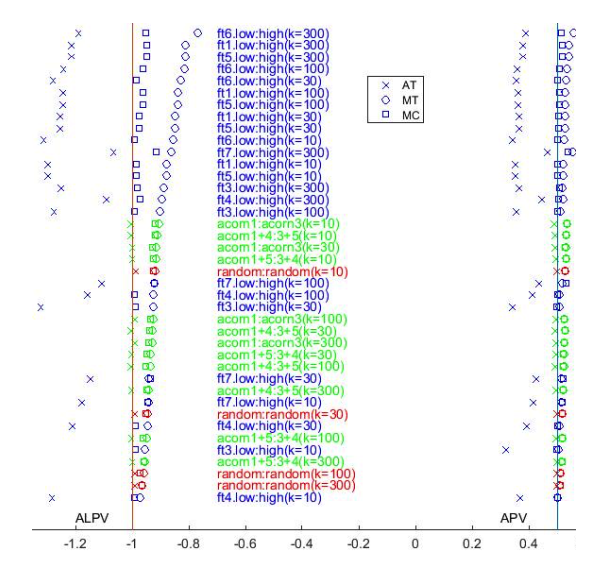
The output of experiments is presented in Ta-bles 1,2,3 and in Figure 1 in graphical form.

Below we analyse the experimental results from these Tables.

Size	Split	CM		AT	MT	MC
1000	Low feature 1	k = 300	APV	0.378	0.542	0.518
	High feature 1	kNN	ALPV	-1.215	-0.812	-0.948
1000	Low feature 1	k = 100	APV	0.363	0.528	0.510
	High feature 1	kNN	ALPV	-1.244	-0.840	-0.962
1000	Low feature 1	k = 30	APV	0.365	0.529	0.505
	High feature 1	kNN	ALPV	-1.255	-0.848	-0.976
1000	Low feature 1	k = 10	APV	0.352	0.522	0.503
	High feature 1	kNN	ALPV	-1.299	-0.879	-0.986
1000	Low feature 3	k = 300	APV	0.364	0.518	0.507
	High feature 3	kNN	ALPV	-1.253	-0.888	-0.980
1000	Low feature 3	k = 100	APV	0.354	0.512	0.501
	High feature 3	kNN	ALPV	-1.276	-0.902	-0.991
1000	Low feature 3	k = 30	APV	0.340	0.508	0.500
	High feature 3	kNN	ALPV	-1.320	-0.925	-0.989
1000	Low feature 3	k = 10	APV	0.318	0.504	0.500
	High feature 3	kNN	ALPV	-1.397	-0.954	-0.989
1000	Low feature 4	k = 300	APV	0.446	0.522	0.506
	High feature 4	kNN	ALPV	-1.090	-0.895	-0.971
1000	Low feature 4	k = 100	APV	0.411	0.510	0.502
	High feature 4	kNN	ALPV	-1.158	-0.924	-0.990
1000	Low feature 4	k = 30	APV	0.393	0.507	0.501
	High feature 4	kNN	ALPV	-1.210	-0.945	-0.987
1000	Low feature 4	k = 10	APV	0.369	0.503	0.501
	High feature 4	kNN	ALPV	-1.283	-0.971	-0.990
1000	Low feature 5	k = 300	APV	0.378	0.542	0.518
	High feature 5	kNN	ALPV	-1.215	-0.812	-0.948
1000	Low feature 5	k = 100	APV	0.363	0.528	0.510
	High feature 5	kNN	ALPV	-1.244	-0.840	-0.962
1000	Low feature 5	k = 30	APV	0.365	0.529	0.505
	High feature 5	kNN	ALPV	-1.255	-0.848	-0.976
1000	Low feature 5	k = 10	APV	0.352	0.522	0.503
	High feature 5	kNN	ALPV	-1.299	-0.879	-0.986
1000	Low feature 6	k = 300	APV	0.390	0.560	0.514
	High feature 6	kNN	ALPV	-1.189	-0.769	-0.952
1000	Low feature 6	k = 100	APV	0.360	0.535	0.509
	High feature 6	kNN	ALPV	-1.243	-0.815	-0.962
1000	Low feature 6	k = 30	APV	0.355	0.532	0.503
	High feature 6	kNN	ALPV	-1.279	-0.827	-0.986
1000	Low feature 6	k = 10	APV	0.342	0.524	0.502
	High feature 6	kNN	ALPV	-1.312	-0.856	-0.990
1000	Low feature 7	k = 300	APV	0.465	0.556	0.538
	High feature 7	kNN	ALPV	-1.065	-0.861	-0.914
1000	Low feature 7	k = 100	APV	0.436	0.520	0.532
	High feature 7	kNN	ALPV	-1.109	-0.922	-0.920
1000	Low feature 7	k = 30	APV	0.425	0.516	0.523
	High feature 7	kNN	ALPV	-1.147	-0.940	-0.934
1000	Low feature 7	k = 10	APV	0.415	0.515	0.517
	High feature 7	kNN	ALPV	-1.178	-0.942	-0.946

Table 3: Results: split by features

INPUT: proper training set w₁; : : : ; w_h

INPUT: calibratlion set z₁; : : : ; z_l

INPUT: testing example z_l+1

INPUT: number k of neighbours

FOR i = 1; : : : ; l + 1

FOR j = 1; : : : ; h

dij = jzi   wj j2

END FOR

let di0

1; : : : ; dih0 be di1; : : : ; dih sorted in ascending order

i =

1

di01+  +dik0

END FOR

cardfi=1;:::;l+1: i   l+1g

OUTPUT p(z

l+1

) =

l+1

Table 4: Scheme of ICP

Set

Size

Generating distribution

Proper training set 1

h

P1h

Calibration set 1

h

P1h

Proper training set 2

h

P2h

Calibration set 2

h

P h

2

2h

P1

+

Testing set

2h

P2

2

Table 5: Experimental setting for ICP

5.2    Effect of data split

For homogeneous split (Table 1) AT approach is (up to the precision) exactly valid in terms of APV. How-ever AT-ALPV in all cases is slightly smaller than -1, this still shows slight conservativeness concentrated for small levels of significance. This may be the topic of a future special study, concentrated on homoge-neous case.

In the other experiments (Tables 2 and 3) we have to analyse invalidity effects for AT. Recall that inva-lidity means that AT-APVs are smaller than ¹₂ or AT-ALPVs are smaller than 1. In Table 3 these devia-tions are much larger, because these splits was done in a more radically way, forced to be heterogeneous, while in Table 2 there are more natural, practical splits.

Comparing the splits from Table 3 to each other, we can see that for some of the features (1,2,5) the de-viations are larger than for the others. This indirectly shows the importance of these features in terms their high influence on the other features. Features (4,7) with relatively small deviation are more random and isolated from the others.

caught by all 36 AT-APV being smaller than 0.5, and in 31 experiments is also confirmed by AT-ALPV being smaller than -1.

• MT and MC are conservatively valid in all the experiments.
• the conservativeness of MC is smaller than MT in 30 experiments, equal (up to the precision) in 2 experiments, and larger in 4 experiments (by APV); smaller in 34 experiments and larger in 2 (by ALPV).

5.4    APV and ALPV criteria

As discussed above, ALPV criterion gives preference to small values of the significance level, because such values are usually applied in the practice. So devia-tions according to ALPV are in principle more critical.

Let us summarise the points where the conclusions slightly differ for these two criteria.

• In homogeneous case, ALPV was more sensitive in catching conservativeness, while APV did not catch any deviation from exact validity.

5.3    Effect of merging approach

As it is seen from Table 1, in case of a purely homo-geneous (random) split the best way of aggregating p-values is just averaging them (AT), the two others are more conservative.

Two other Tables 2 and 3) contain 36 comparisons of AT, MT and MC approaches. They show is follow-ing:

• AT is invalid in all the experiments. This is
• On the other hand, in catching invalidity (as seen in heterogeneous case) APV is stronger.
• Being more sensitive for conservativeness, ALPV better shows advantages of MC over MT in decreasing its level.

All this reflects that the damage from conserva-tiveness is more concentrated in small significance levels, when CP is distributed for big data.

Average p-Value						Average Logarithm p-Value		Interpretation
<		1				<	1	invalid
		2
=			1			=	1	valid and efficient
			2
>	1					>	1	valid but conservative
2

Table 6: Understanding the results of evaluation

5.5    Effect of CM choice

This work concentrates on the effects of conservative-ness and does not aim to answer in general the ques-tion which CM is better for the specific problem of anomaly detection. As mentioned above, the full an-swer actually can be done based either on an addi-tional testing set of known anomalies, or on a measure on the whole objects space, which may depend on the physical meaning of the data.

Here we just make preliminary notes about influ-ence of the parameter k (number of nearest neigh-bours) on the conclusion. Usually the larger this num-ber is, the more centered/unified is the notion of nor-mal (not abnormal) behaviour, less splitter into sepa-rate behaviour types.

• In homogeneous case (Table 1), conservativeness (of AT) increases for the small values of neigh-bour number k.
• In heterogeneous case (Tables 2-3), validity (of AT) is also a larger problem for small k.
• Conservativeness of MT is larger for small k when the split is moderately heterogeneous (Ta-ble 2) and for large k when the split is more het-erogeneous (Table 3).
• Advantage of replacing MT by MC is smaller for large k.

6. Discussion

6.1    Conclusion

In this work we suggest a MC way of aggregation of p-values for Conformal Prediction that is the best mid-dle way between invalid averaging and conservative maximization of partial p-value obtained from differ-ent data sources. This method is applicable on big and heterogeneously split data.

It advantage was shown in Section 3 theoretically in an asymptotical sense, and confirmed on the ex-perimental part on real data. The validity property is kept, while the conservativeness is essentially smaller than for aggregating p-values by maximizing them in most of the cases.

6.2    Future work

For the future work, we can mention the following points.

First, the general case presented in Proposition 1 (see Section 3.8) is applicable as well to a more gen-eral case of several sources of different size, this also is interesting to be checked practically.

Second, the area of application used in this paper was detection of anomalies behaviour of households. An interesting related area where these ideas may be applied in the future is growing area of internet of things such as medical sensors. Anomaly behaviour of users is an actual thing to be detected. The practice shows that the alarm/alert criteria have to be based on the analysis of essential data collections, otherwise they may be too approximate in a specific patient’s situation.

Third, it was discussed in the work that this frame-work is transferrable from anomaly detection to su-pervised learning where validity of prediction sets is important as well. This opens many more applica-tions. But there is a challenge of the following type. In a supervised learning task, the validity and con-servativeness is determined by p-values assigned to true hypotheses about the labels of new data exam-ples. It can be measure by analogy to this paper, but what about hypotheses assigned to wrong hypotheses? The conformal supervised learning is the more effi-cient the smaller are these p-values. The best situation is when p-values for all hypotheses except the true one are small (close to 0). This property may be also affected on the aggregated stage, where the p-values tend to increase, so theoretical and/or experimental validation has to ensure that it is not lost.

Conflict of Interest

Authors declare no conflict of interest.

Acknowledgments

This work was supported by Technology Integrated Health Management (TIHM) project awarded to the School of Mathematics and Information Security at Royal Holloway as part of an initiative by NHS England supported by Innova-teUK. It was also supported by European Union grant 671555 (”ExCAPE”), EPSRC grant EP/K033344/1 (”Mining the Network Behaviour of Bots”), Thales grant (”Development of automated methods for de-tection of anomalous behaviour”), and by the National Natural Science Foundation of China (No.61128003) grant.

The large help for this work was done to Lars Carlsson. He gave us the initial motivation for the work, stating the problem of conservativeness in the case of homogeneous split. Another motivation came from the area of aggregating results of different prediction algorithms. In particular it was inspired by recent works [12] with application of CP to big data. and [13] covering the theme of merging data splits as well as merging prediction algorithms. We are grate-ful to Paolo Toccaceli, Vladimir Vovk, Alex Gammer-man and Zhiyuan Luo for useful discussions in this area.

TIHM project directed our attention to anomalies in behaviour-related practical problems as an area of application. We are especially grateful to Energy De-mand Research Project for providing the data.

1. I. Nouretdinov. “Distributed conformal anomaly detection” in 15th IEEE International Conference on Machine Learning and Applications, Anaheim USA, 2016.
2. V. Vovk, A. Gammerman, G. Shafer. “Algorithmic learning in a random world” Springer, 2005
3. V. Vovk, V. Fedorova, I. Nouretdinov, A. Gammerman. “Criteria of efficiency for conformal prediction” in Conformal and Probabilistic Prediction with Applications: 5th International Symposium, Madrid Spain, 2016.
4. R. Laxhammar, G. Falkman. “Sequential conformal anomaly detection in trajectories based on Hausdorff distance” in 14th International Conference on Information Fusion, Chicago USA, 2011.
5. R. Laxhammar. “Conformal anomaly detection. Detecting abnormal trajectories in surveillance applications” Ph.D Thesis. University of Skovde, ¨ Sweden, 2014.
6. J. Smith, I. Nouretdinov, R. Craddock, C. Offer, A. Gammerman. “Anomaly detection of trajectories with kernel density estimation by conformal prediction” in Artificial Intelligence Applications and Innovations, Rhodes Greece, 2014.
7. J. Smith, I. Nouretdinov, R. Craddock, C. Offer, A. Gammerman. “Conformal anomaly detection of trajectories with a multi-class hierarchy” in Statistical Learning and Data Sciences: Third International Symposium, Egham UK, 2015.
8. J. Smith. “The efficiency of conformal prediction for anomaly detection” PhD thesis. Royal Holloway University of London, UK, 2016.
9. G. Cherubin, I. Nouretdinov, A. Gammerman, R. Jordaney, Z. Wang, D. Papini, L. Cavallaro. “Conformal clustering and its application to botnet traffic” in Statistical Learning and Data Sciences: Third International Symposium, Egham UK, 2015.
10. V. Fedorova, A. Gammerman, I. Nouretdinov, V. Vovk. “Plug-in martingales for testing exchangeability on line” in 29th International Conference on Machine Learning, Edinburgh UK, 2012.
11. H. Graf, E. Cosatto, L. Bottou, I. Durdanovic, V. Vapnik. “Parallel support vector machines: the cascade SVM” in Advances in Neural Information Processing Systems 17, Vancouver Canada, 2004.
12. P. Toccaleli, I. Nouretdinov, A. Gammerman. “Conformal predictors for compound activity prediction” in Conformal and Probabilistic Prediction with Applications: 5th International Symposium, Madrid Spain, 2016.
13. V. Vapnik, R. Izmailov. “Synergy of monotonic rules” J. Mach. Learn. Res., 17(136), 1–33, 2016.

(Click to view)

(Click to view)