Schizophrenia Prediction Using Integrated Imaging Genomic Networks

1 Introduction

This paper is an extension of work originally presented in the IEEE International Conference on Bioinformatics and Biomedicine (BIBM 2016) [1].

Currently, there is a lack of objective ways for the diagnosis of schizophrenia (SCZ) [2]. It is generally diagnosed according to criteria set in either the American Psychiatric Associations fifth edition of the Diagnostic and Statistical Manual of Mental Disorders (DSM 5), or the World Health Organizations International Statistical Classification of Diseases and Related Health Problems (ICD-10). These criteria use the self-reported experiences of the patients and report abnormalities in their behaviors, followed by a clinical assessment by a mental health professional. However, symptoms associated with schizophrenia occur along a continuum in the population and must reach a certain severity before a diagnosis is made [3]. Although in psychiatry as in all of general medicine there is an irreducible element of the subjective [4], we should try our best to reduce the subjective part of medical and psychiatry practice. This goal is well recognized by the National Institutes of Mental Health as well [5].

Like many other complex diseases, SCZ is caused by a combination of genetic, biological, and environmental factors, creating a difficult challenge for diagnosis and defining subtypes. In addition, SCZ is a highly heritable disorder [6]. The current belief is that there are a number of genes that contribute to susceptibility or pathology of SCZ, but none of them exhibits full responsibility for the disease. It is believed that SCZ is caused by a number of genetic and environmental factors [7].

Recently, high-throughput studies are rapidly accumulating a wealth of ’omics’-scale data, which enable comprehensive monitoring of a biological system. Meanwhile, there are remarkable medical images accumulated in hospitals, such as images from functional magnetic resonance imaging (fMRI). fMRI is a fairly new tool that has been used to measure brain activation utilising the dependency of the magnetic properties of haemoglobin on the amount of oxygen it carries. Blood-oxygen-level-dependent (BOLD) signals measure the alterations in cerebral blood flow that mark functional brain activity [8]. The intrinsic BOLD contrast makes fMRI an invaluable noninvasive instrument for the investigation of the underlying physiological disturbances that lead to manifest psychiatric disorders. It is anticipated that successful application and analysis of fMRI in neurological disorders can be used to characterise and diagnose mental illnesses such as Alzheimers disease, SCZ, bipolar disorder, mild traumatic brain injury and addiction. It is a valuable way to combine genetic, epigenetic and imaging data for the diagnosis of SCZ disease. Many studies have demonstrated that the integration of fMRI and SNP information will give a more comprehensive analysis of schizophrenia. For example, Yang et al. [9] proposed a hybrid machine learning method to identify schizophrenia patients from healthy controls by combining genetic and fMRI data, and this method achieved better classification accuracy than using either data alone. Castro et al. [10] developed a multiple kernel learning approach that employed both the phase and the magnitude of complex-valued fMRI data for the classification, showing improved classification accuracy compared with using only the magnitude of fMRI data. Cao et al. proposed a sparse representation clustering (SRC) model [11, 12] to simultaneously select SNPs and fMRI voxels as biomarkers for schizophrenia followed by a classifier such as support vector machine (SVM). The integrative model was tested on 20 SCZ patients and 20 healthy controls, demonstrating that the complementary information from both fMRI and SNP data can be utilized to improve diagnosis [13].

The above mentioned SCZ studies, however, only used two types of data: SNPs and fMRI data. DNA methylation is one of several epigenetic mechanisms and can be used by cells to control gene expression. There are a number of mechanisms controlling gene expression in eukaryotes, but DNA methylation is a frequently used epigenetic signaling tool, which can fix genes in the “off “ position [14]. In addition, the integration methods used in the above mentioned research directly used features extracted from data as predictors. Alternatively, network-based classification methods mainly employ the topological features as predictors. With the rapid development of systems biology, network-based classification or prediction methods have been widely used [15, 16, 17, 18, 19, 20, 21].

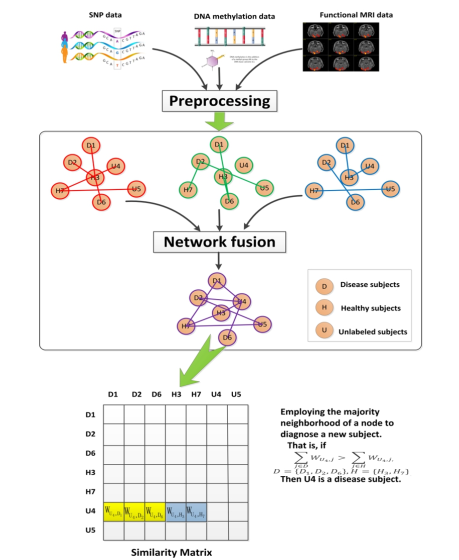
In our study, we combined three types of data including SNPs, DNA methylation and fMRI to construct networks, which were subsequently be fused for diagnosis of SCZ. Specifically, for each type of data, we first constructed a patient network, called a single network. Thus for three types of data, we constructed three single networks. Then we fused two or three single patient networks into one subject network. As a result, we created four fused networks: three fused networks from the combinations of two data types and one fused network from three data types. Finally, we employed the neighborhood majority of the nodes in the network to predict unknown labels, that is, identifying whether a subject is a schizophrenia patient.

2 Data Preparation

In this study, participant recruitment and data collection were conducted at the Mind Research Network. Three types of data (SNP, DNA methylation and fMRI) were collected from 208 subjects including 96 schizophrenia patients (age: 34 ± 11, 22 females) and 112 healthy controls (age: 32 ± 11, 44 females). All of them were provided written informed consents. Healthy participants were free of any medical, neurological or psychiatric illnesses and had no history of substance abuse. By the clinical interview of patients for DSM IV-TR Disorders or the Comprehensive Assessment of Symptoms and History, patients met criteria for DSM-IV-TR schizophrenia. Antipsychotic history was collected as part of the psychiatric assessment. After a series of quality controls, we selected 184 subjects, including 80 SZ cases (age: 34 ± 11, 20 females and 60 males) and 104 healthy controls (age:32 ± 11, 38 females and 66 males). After pre-processing, 27,508 DNA methylation sites, 41,s236 fMRI voxels and 722,177 SNP loci were obtained for the subsequent biomarker selections [22, 23, 24, 25, 26, 27].

2.1     SNPs data collection and preprocessing

A blood sample was obtained for each participant and DNA was extracted. Genotyping for all participants was performed at the Mind Research Network using the Illumina Infinium HumanOmni1-Quad assay covering 1,140,419 SNP loci. Bead Studio was used to make the final genotype calls. Next, the PLINK software

package(http://pngu.mgh.harvard.edu/∼purcell/plink) was used to perform a series of standard quality control procedures, resulting in the final dataset spanning 722,177 SNP loci. Each SNP was categorized into three clusters based on their genotype and was represented with discrete numbers: 0 for ‘BB‘(no minor allele), 1 for ‘AB‘ (one minor allele) and 2 for ‘AA‘ (two minor alleles).

2.2     DNA methylation data collection and preprocessing

DNA from blood samples was assessed by the Illumina Infinium Methylation27 Assay. A methylation value, beta (β), represents the ratio of the methylated probe intensity to the total probe intensity. A series of quality controls (QC) on the beta values were applied to remove bad samples and probes, such as 1) Beta value QC: Change any beta value to NaN, if p>0.05. 2) Bad sample/ bad marker removing: Samples with >5% of missing (NaN) values; markers with >5% of missing (NaN) values. This resulted in the identification of good methylation data from 224 subjects, 27,508 markers (some have missing values <5%). After QC, we used the K nearest neighbor (KNN) method [28]to impute for the missing values.

2.3     fMRI data collection and preprocessing

The fMRI data were collected during a sensorimotor task, a block-design motor response to auditory stimulation. During the on-block, 200msec tones were presented with a 500 msec stimulus onset asynchrony (SOA). A total of 16 different tones were presented in each on-block, with frequency ranging from 236 Hz to 1318 Hz. The fMRI images were acquired on Siemens 3T Trio Scanners and a 1.5T Sonata with echo-planar imaging (EPI) sequences using the following parameters (TR = 2000 msec, TE = 30 msec (3.0T)/40 msec (1.5T), field of view = 22cm, slice thickness = 4mm, 1mm skip, 27 slices, acquisition matrix = 64 × 64, flip angle =90^◦.). Data were pre-processed in SPM5 (http://www.fil.ion.ucl.ac.uk/spm) and were realigned, spatially normalized and resliced to 3×3× 3mm³, smoothed with a 10×10×10mm³ Gaussian kernel to reduce spatial noise, and analyzed by multiple regression considering the stimulus and their temporal derivatives plus an intercept term as regressors. Finally the stimulus-on versus stimulus-off contrast images were extracted with 53×63×46 voxels and all the voxels with missing measurements were excluded.

3 Methods

3.1      Overview

We employed a network-based semi-supervised learning (SSL) scheme, which improves the predictive power by using unlabeled data [29, 30, 31, 32]. It is compuationally efficient and the learning time depends nearly linearly on the number of network edges. Also, the accuracy is comparable with other methods such as kernel-based methods with a longer learning time [18, 33]. Moreover, the network structure can facilitate the interpretation of gene-gene interactions and/or region- region connections in the brain [34, 35, 36], which is one of the advantages of network-based SSL.

Based on a fused network, our label prediction method mainly consists of three procedures: network construction, network fusion and label prediction using network-derived features.

3.2       Network Construction

Based on the features selected from SNPs, DNA methylation and fMRI data, a subject network can be constructed. Suppose we have n samples and m measurements (e.g., DNA methylation). A subject similarity network is represented as a graph G = (V,E). The vertices V correspond to the subjects {x₁,x₂,…,x_n} and the strengths of the edges E are the weighted value of the similarity between subjects. The edge weights are represented by an n × n similarity matrixW, with each W_ij indicating the similarity between subjects x_i and x_j. ρ₍x_i,x_j) is represented as the Euclidean distance between subjects x_i and x_j. In order to calculate edge strength, a Gaussian function was taken on the Euclidean distance between subjects:

Wij = _ exp(−               _σi,x2j)2),       if i ∼ j     (1) ρ(x

                             _^ 0.                            otherwise

0

If i is in j s K-nearest-neighborhood and vice versa, nodes i,j can be connected by an edge. In our study, we constructed three individual networks for SNPs, DNA methylation, and fMRI data.

3.3       Network Fusion

We fuse multiple networks into one network, using mean fusion in our study. Multiple networks, denoted by G^m = (V ^m,E^m,w^m),m = 1,2,3,…,N, are constructed from multiple types of data. They have the same network nodes and the edge strength in the fused network is the mean value of edge strength of all individual networks.

G = (V ,E,w), with V = ∪_mV ^m,E = ∪_mE^m,

N and w(i,j) = 1 ^Xw^m(i,j).       (2)

N

m=1

Using this graph fusion method, we fused two or three single patient networks into one subject network. As a result, we created four fused networks: three fused networks from the combinations of two data types and one fused network for three data types.

3.4 Label Prediction Based on Neighborhood Majority

A network is a map of interactions, with the links measuring the association between objects or subunits. A labeled subject is marked either by 0 or 1, representing two possible labels: healthy or disease, respectively. The edges have an essential role in influencing the propagation between the subjects to predict the true label of the unknown subject. We assumed that the labels of two subjects are more likely to be the same if the two subjects are more closely related to each other. Therefore, the labels can be predicted based on the similarities between subjects with their genomic profiles and/or imaging features. Edges in network-based SSL represent the similarities between subjects that can be extracted from different data including SNPs, DNA methylation and fMRI data

(Figure).

Network-based classification methods can be classified into two types [21]: direct annotation schemes, which infer the class label of a node based on its connections in the network, and module-assisted schemes, which first identify modules of related nodes and then annotate each module based on the known labels of its members. Neighborhood counting is a simple and direct method for label prediction, which determines the label of a subject based on the known label of subjects lying in its immediate neighborhood. Here, we used neighborhood majority to predict the unknown labels. We first calculated the neighborhood majority of a query subject. Then, the subject is assigned the same type of label as the one of its immediate neighbors with greatest neighborhood majority (Figure).

For a query subject i, the majority of its immediate neighbors can be defined as:

N_k

X

                                         M_k =         W_ij                                                       (3)

j=1

where k represents subject class index and N_k is the number of subjects in class k. Then the label of subject i is defined as:

y(i) = y(arg maxM_k)             (4) k

4 Results and Discussions

We employed a network-based classification method to predict whether new subjects are schizophrenia patients. After preprocessing the three types of collected data: SNPs, DNA methylation and function MRI data, we chose 184 subjects with all three types of data. We used 5-fold cross validation to evaluate our prediction method. A two-step feature selection method was applied to the labeled data sets. At first, for SNPs and DNA methylation data sets, we preselected the features based on the genes in KEGG pathways and this procedure yielded 14,875 SNPs and 6,935 DNA methylation sites. Then, for three types of data, we utilized the t-test to select the significantly differential features (p≤0.01) between normal and disease status. The preselected features were used to construct a subject-subject network. A single-type network was built for each data type. That is, three single-type networks were generated. Next, a network fusion method was used to build fused networks from two or three single-type networks. Thus we can get four fused networks: three fused networks from the pairwise combinations of two data types and one fused network from three data types. In our previous study [37], it has been shown that the technique of data fusion will improve the classification performance of network based classifiers. Therefore, in this paper, we focus on the study of the fused network from three types of data. Based on the fused network, we utilized nodes’ features in a network to predict the label of a testing subject. This process is illustrated in Figure. Our prediction method is called MMN, which is a majority-neighborhood-based classification method by mean fusion.

We also compared the performance of our model with that of several other network based classification methods, with fixed parameter settings (σ² = 510,andK = 20). We compared 10 network based methods, whose differences consist in the procedure of network fusion and the algorithm of classification. For network fusion, two alternative methods are the mean fusion as used by our model, and Similarity Network Fusion (SNF) [38]. For classification procedure, we used five different classification methods: majority-neighborhood based classification (MN), which is adopted by our model, spectral clustering (SPC) [39, 40], support vector machine (SVM) [41], local and global consistency (LGC) [32], and label propagation (LP) [42]. SPC is a module-assisted classification approach based on spectral clustering, which is efficient in capturing global structure of a graph [43]. SVM utilizes 11 node features extracted from the network for label classification, and these 11 node features are: betweenness centrality, closeness centrality, degree centrality, Bonacich Power centrality scores, the (Harary) graph centrality, information centrality, the load centrality, the vertex prestige scores, the stress centrality, and clustering coefficients [44]. LGC utilizes both the local and the global consistency of a new patient in a patient-patient network for classification. LP predicts the clinical outcome of the new patient based on a network structure called label propagation. Thus, we have 10 different models, which are MMN (our model), SMN, MSPC, SSPC, MSVM, SSVM, MLGC, SLGC, MLP, and SLP, respectively. To evaluate the performances of these 10 network-based label prediction methods, we computed some widely used metrics, e.g., true positive rate (TPR), true negative rate (TNR), negative predictive value (NPV), false positive rate (FPR), false negative rate (FNR), false discovery rate (FDR), accuracy (ACC), and F1 (F1 = 2TP/2TP+FP+FN) of each method. The classification performances of all these models are listed in Table 1.

From these results it is evident that our model, MMN performs significantly better than other network based classification methods, in terms of some key metrics, e.g. ACC, FDR, etc. Also, it seems that those mean fusion based methods (MLP, MLGC, MMN, MSPC, MSVM) works slightly better than thef corresponding SNF based methods (SLP, SLGC, SMN, SSPC, SSVM), which demonstrates the advantage of mean fusion over SNF. In summary, mean fusion is more suitable than SNF for classification, and MMN works significantly better than other graph-based

Table 1: The performances of different graph-based label prediction methods Methods TPR TNR NPV FPR FNR FDR ACC SLP 1 0 NA 1 0 0.568 0.432 MLP 1 0 NA 1 0 0.568 0.432 SLGC 1 0 NA 1 0 0.568 0.432 MLGC 1 0 NA 1 0 0.568 0.432 SMN 0 1 0.568 0 1 NA 0.568 MMN 0.588 0.756 0.698 0.244 0.412 0.332 0.686 SSPC 0 1 0.568 0 1 NA 0.568 MSPC 0.338 0.726 0.6 0.274 0.662 NA 0.556 SSVM 0 1 0.56 0 1 NA 0.56 MSVM 0.388 0.754 0.614 0.246 0.612 0.424 0.598 Table 2: The performances of our label prediction method MMN with different σ2(K = 20) σ2 TPR SPC NPV FPR FNR FDR ACC F1 100 0.54 0.688 0.65 0.312 0.464 0.408 0.624 0.566 150 0.54 0.688 0.65 0.312 0.464 0.408 0.624 0.576 200 0.564 0.716 0.672 0.284 0.438 0.374 0.65 0.582 250 0.552 0.726 0.674 0.274 0.45 0.378 0.652 0.592 300 0.564 0.746 0.684 0.254 0.438 0.352 0.668 0.603 350 0.564 0.746 0.684 0.254 0.438 0.352 0.668 0.598 400 0.564 0.756 0.686 0.244 0.438 0.342 0.674 0.607 450 0.564 0.756 0.686 0.244 0.438 0.342 0.674 0.602 500 0.588 0.756 0.698 0.244 0.412 0.332 0.686 0.625 510 0.603 0.758 0.707 0.242 0.399 0.329 0.694 0.630 520 0.612 0.746 0.71 0.254 0.388 0.336 0.692 0.632 530 0.612 0.746 0.71 0.254 0.388 0.336 0.69 0.632 540 0.612 0.738 0.708 0.282 0.388 0.366 0.686 0.628 550 0.612 0.738 0.708 0.262 0.388 0.346 0.684 0.628 560 0.612 0.738 0.708 0.262 0.388 0.346 0.686 0.628 570 0.612 0.738 0.728 0.262 0.388 0.344 0.686 0.628 580 0.612 0.738 0.708 0.262 0.388 0.346 0.686 0.628 590 0.612 0.738 0.708 0.262 0.388 0.346 0.686 0.628 600 0.612 0.738 0.708 0.262 0.388 0.346 0.686 0.631 650 0.6 0.738 0.702 0.262 0.402 0.35 0.68 0.620 700 0.6 0.738 0.702 0.262 0.394 0.346 0.68 0.624 750 0.6 0.738 0.702 0.262 0.402 0.35 0.68 0.620 800 0.588 0.738 0.694 0.262 0.414 0.352 0.674 0.617 850 0.588 0.738 0.694 0.262 0.414 0.352 0.674 0.612 900 0.588 0.728 0.692 0.272 0.414 0.364 0.668 0.611 950 0.588 0.728 0.692 0.272 0.414 0.364 0.67 0.608

methods.

At first, we want to compare two different network fusion methods: mean fusion and SNF [38]. For each classification approach, we used both network fusion methods. So according to the network fusion, the 10 prediction methods implemented in our study are all grouped into pairwise comparisons. For example, in SLP and MLP, the first letter S in the method symbol SLP denotes SNF fusion method and the first M in the method symbol MLP means mean fusion approach. It is the same for other pairs of prediction methods:

Table 3: The performances of our label prediction method MMN with different K(σ2 = 510) K TPR SPC NPV FPR FNR FDR ACC F1 37 0.513 0.708 0.648 0.292 0.488 0.41 0.625 0.546 20 0.603 0.758 0.707 0.242 0.399 0.329 0.694 0.630 18 0.563 0.727 0.678 0.273 0.438 0.371 0.657 0.592 12 0.538 0.728 0.67 0.272 0.463 0.389 0.646 0.57 9 0.525 0.752 0.665 0.248 0.475 0.347 0.654 0.578 7 0.538 0.742 0.669 0.258 0.463 0.34 0.656 0.581 Figure 1 The Schematic of Schizophrenia Diagnosis

SLGC and MLGC, SMN and MMN, SSPC and MSPC, SSVM and MSVM. Table 1 shows the performances of different prediction algorithms between two network fusion methods. As can be seen in Table 2, for the prediction methods based on LP and LGC, there are no differences in performances between two network fusion approaches. For SSPC and MSPC, the only one group of module-assisted prediction methods, their accuracies are close to each other and neither got good performance. The results are similar to another pair of prediction methods: SSVM and MSVM. The major difference between SPC-based pair is that the mean-fusion-based method MSVM obtained higher accuracy than SNF-based method SSVM. However, the comparison results between SMN and MMN differ greatly from other graph-based prediction method pairs. For each of the performance metrics, MMN performs better than SMN, especially the ACC. Actually, the network fusion method used in this study uses uniform weight, i.e., equal weight for each of multiple individual networks. In the future, we will try to develop a weighted mean fusion method, which can assign an optimal weight for each individual network.

Above all, our prediction method MMN performs the best among all those graph-based label prediction methods and it is computationally efficient.

When computing the edge strength for constructing networks, there are two parameters σ,K related to the prediction accuracy. When selecting an optimal σ, we fixed the parameter K (K=20) and evaluated the performances with σ² ranging from 100 to 950. The results are shown in Table 2 and we can see that when σ² is too small or too large, the prediction accuracy decreases and MMN performs best with σ² = 510. When selecting an optimal K, σ² was fixed at 510 with K changing in the range 7, 9, 12, 18, 20, 37 corresponding to 1/25, 1/20, 1/15, 1/10, 1/9, 1/5 of the number of the samples. As shown in Table 3, our methods achieves the best accuracy with K = 20, which is about 1/10 of whole sample (nodes) size.

5 Conclusions

We combined SNPs, DNA methylation and fMRI data into a single comprehensive network using a simple network fusion approach. A network-based label prediction method was applied to the network for predicting schizophrenia patient. Compared with other 9 graph-based label prediction approaches, our prediction method shows the best performance. However, our network fusion method used a uniform weight based combination of each network and in the future we will find an optimal weight based method to improve the prediction accuracy. In addition, Kim et al.[19] incorporated genomic knowledge when integrating multi-omics data for predicting the clinical outcome of cancer, which improved the predictive power. Therefore, we will also incorporate other prior knowledge into the construction of patient connection networks.

Conflict of Interest The authors declare no conflict of interest.

Acknowledgment The work are partly supported by the grants: the NIH (R01 GM109068, R01 MH104680, and R01MH107354) and NSF (#1539067). China Postdoctoral Science Foundation Grant, No. 2015M580352.

1. S.-P. Deng, D. Lin, V. D. Calhoun, and Y.-P. Wang, “Diagnosing schizophrenia by integrating genomic and imaging data through network fusion,” in Bioinformatics and Biomedicine (BIBM), 2016 IEEE International Conference on. IEEE, 2016, pp. 1307–1313.
2. A. P. Association et al., Diagnostic and statistical manual of mental disorders (DSM-5®). American Psychiatric Pub, 2013.
3. M. M. Picchioni and R. M. Murray, “Schizophrenia,” BMJ, vol. 335, no. 7610, 2007.
4. R. Pies, “How objective are psychiatric diagnoses,” Psychiatry, vol. 4, no. 10, 2007.
5. T. Insel, B. Cuthbert, M. Garvey, R. Heinssen, D. S. Pine, K. Quinn, C. Sanislow, and P. Wang, “Research domain criteria (rdoc): toward a new classification framework for research on mental disorders,” American Journal of Psychiatry, vol. 167, no. 7, pp. 748–751, 2010.
6. S. Ripke, B. M. Neale, A. Corvin, J. T. Walters, K.- H. Farh, P. A. Holmans, P. Lee, B. Bulik-Sullivan, D. A. Collier, H. Huang et al., “Biological insights from 108 schizophrenia-associated genetic loci,” Nature, vol. 511, no. 7510, p. 421, 2014.
7. A. P. M. M. S. Owen, Schizophrenia. London, England: Lancet, 2016.
8. S. Ogawa, T.-M. Lee, A. R. Kay, and D. W. Tank, “Brain magnetic resonance imaging with contrast dependent on blood oxygenation,” Proceedings of the National Academy of Sciences, vol. 87, no. 24, pp. 9868–9872, 1990.
9. H. Yang, J. Liu, J. Sui, G. Pearlson, and V. D. Calhoun, “A hybrid machine learning method for fusing fmri and genetic data: combining both improves classification of schizophrenia,” Frontiers in human neuroscience, vol. 4, p. 192, 2010.
10. E. Castro, V. Gómez-Verdejo, M. Martínez Ramón, K. A. Kiehl, and V. D. Calhoun, “A multiple kernel learning approach to perform classification of groups from complex-valued fmri data analysis: Application to schizophrenia,” NeuroImage, vol. 87, pp. 1–17, 2014.
11. H. Cao, J. Duan, D. Lin, V. Calhoun, and Y.- P. Wang, “Integrating fmri and snp data for biomarker identification for schizophrenia with a sparse representation based variable selection method,” BMC medical genomics, vol. 6, no. Suppl 3, p. S2, 2013.
12. H. Cao, D. Lin, J. Duan, Y.-P. Wang, and V. Calhoun, “Bio marker identification for diagnosis of schizophrenia with integrated analysis of fmri and snps,” in Bioinformatics and Biomedicine (BIBM), 2012 IEEE International Conference on. IEEE, 2012, pp. 1–6.
13. D. Lin, H. Cao, Y.-P. Wang, and V. Calhoun, “Classification of schizophrenia patients with combined analysis of snp and fmri data based on sparse representation,” in Bioinformatics and Biomedicine (BIBM), 2011 IEEE International Conference on. IEEE, 2011, pp. 394–397.
14. S. Robertson, “What is dna methylation?” new Medical. [Online]. Available: http://www.news-medical.net/life-sciences/What-is-DNA-Methylation.aspx
15. T. Shlomi, M. N. Cabili, M. J. Herrgrd, B. Ø. Palsson, and E. Ruppin, “Network-based prediction of human tissue-specific metabolism,” Nature biotechnology, vol. 26, no. 9, pp. 1003–1010, 2008.
16. H.-Y. Chuang, E. Lee, Y.-T. Liu, D. Lee, and T. Ideker, “Network-based classification of breast cancer metastasis,” Molecular systems biology, vol. 3, no. 1, p. 140, 2007.
17. L. Q. Uddin, K. Supekar, C. J. Lynch, A. Khouzam, J. Phillips, C. Feinstein, S. Ryali, and V. Menon, “Salience network–based classification and prediction of symptom severity in children with autism,” JAMA psychiatry, vol. 70, no. 8, pp. 869–879, 2013.
18. K. Tsuda, H. Shin, and B. Scholkopf, “Fast protein classification with multiple networks,” Bioinformatics, vol. 21, no. suppl 2, pp. ii59–ii65, 2005.
19. D. Kim, J.-G. Joung, K.-A. Sohn, H. Shin, Y. R. Park, M. D. Ritchie, and J. H. Kim, “Knowledge boosting: a graph-based integration approach with multi-omics data and genomic knowledge for cancer clinical outcome prediction,” Journal of the American Medical Informatics Association, vol. 22, no. 1, pp. 109–120, 2015.
20. D. Kim, H. Shin, Y. S. Song, and J. H. Kim, “Synergistic effect of different levels of genomic data for cancer clinical outcome prediction,” Journal of biomedical informatics, vol. 45, no. 6, pp. 1191–1198, 2012.
21. R. Sharan, I. Ulitsky, and R. Shamir, “Networkbased prediction of protein function,” Molecular systems biology, vol. 3, no. 1, p. 88, 2007.
22. H. Cao, J. Duan, D. Lin, Y. Y. Shugart, V. Calhoun, and Y.-P. Wang, “Sparse representation based biomarker selection for schizophrenia with integrated analysis of fmri and snps,” Neuroimage, vol. 102, pp. 220–228, 2014.
23. D. Lin, J. Zhang, J. Li, H. He, H.-W. Deng, and Y.-P. Wang, “Integrative analysis of multiple diverse omics datasets by sparse group multitask regression,” Multi-omic Data Integration, p. 126, 2015.
24. R. L. Gollub, J. M. Shoemaker, M. D. King, T. White, S. Ehrlich, S. R. Sponheim, V. P. Clark, J. A. Turner, B. A. Mueller, V. Magnotta et al., “The mcic collection: a shared repository of multimodal, multi-site brain image data from a clinical investigation of schizophrenia,” Neuroinformatics, vol. 11, no. 3, pp. 367–388, 2013.
25. J. Liu, J. Chen, S. Ehrlich, E. Walton, T. White, N. Perrone-Bizzozero, J. Bustillo, J. A. Turner, and V. D. Calhoun, “Methylation patterns in whole blood correlate with symptoms in schizophrenia patients,” Schizophrenia bulletin, vol. 40, no. 4, pp. 769–776, 2014.
26. J. Liu, M. Morgan, K. Hutchison, and V. D. Calhoun, “A study of the influence of sex on genome wide methylation,” PloS one, vol. 5, no. 4, p. e10028, 2010.
27. E. Walton, J. Liu, J. Hass, T. White, M. Scholz, V. Roessner, R. Gollub, V. D. Calhoun, and S. Ehrlich, “Mb-comt promoter dna methylation is associated with working-memory processing in schizophrenia patients and healthy controls,” epigenetics, vol. 9, no. 8, pp. 1101–1107, 2014.
28. N. S. Altman, “An introduction to kernel and nearest-neighbor nonparametric regression,” The American Statistician, vol. 46, no. 3, pp. 175–185, 1992.
29. O. Chapelle, J. Weston, and B. Scholkopf, “Cluster kernels for semi-supervised learning,” in Advances in neural information processing systems, 2002, pp. 585–592.
30. X. Zhu, Z. Ghahramani, J. Lafferty et al., “Semisupervised learning using gaussian fields and harmonic functions,” in ICML, vol. 3, 2003, pp. 912–919.
31. M. Belkin, I. Matveeva, and P. Niyogi, “Regularization and semi-supervised learning on large graphs,” in International Conference on Computational Learning Theory. Springer, 2004, pp. 624–638.
32. D. Zhou, O. Bousquet, T. N. Lal, J. Weston, and B. Scholkopf, “Learning with local and global consistency,” Advances in neural information processing systems, vol. 16, no. 16, pp. 321–328, 2004.
33. H. Shin, K. Tsuda, B. Scholkopf, A. Zien et al., “Prediction of protein function from networks,” in Semi supervised learning. MIT press, 2006, pp. 361–376.
34. P. T. Spellman, G. Sherlock, M. Q. Zhang, V. R. Iyer, K. Anders, M. B. Eisen, P. O. Brown, D. Botstein, and B. Futcher, “Comprehensive identification of cell cycle–regulated genes of the yeast saccharomyces cerevisiae by microarray hybridization,” Molecular biology of the cell, vol. 9, no. 12, pp. 3273–3297, 1998.
35. E. Segal, M. Shapira, A. Regev, D. Pe’er, D. Botstein, D. Koller, and N. Friedman, “Module networks: identifying regulatory modules and their condition-specific regulators from gene expression data,” Nature genetics, vol. 34, no. 2, pp. 166–176, 2003.
36. J. H. Ohn, J. Kim, and J. H. Kim, “Genomic characterization of perturbation sensitivity,” Bioinformatics, vol. 23, no. 13, pp. i354–i358, 2007.
37. S.-P. Deng, D. Lin, V. D. Calhoun, and Y.-P. Wang, “Predicting schizophrenia by fusing networks from snps, dna methylation and fmri data,” in Engineering in Medicine and Biology Society (EMBC), 2016 IEEE 38th Annual International Conference of the. IEEE, 2016, pp. 1447–1450.
38. B. Wang, A. M. Mezlini, F. Demir, M. Fiume, Z. Tu, M. Brudno, B. Haibe-Kains, and A. Goldenberg, “Similarity network fusion for aggregating data types on a genomic scale,” Nature methods, vol. 11, no. 3, pp. 333–337, 2014.
39. A. Y. Ng, M. I. Jordan, Y. Weiss et al., “On spectral clustering: Analysis and an algorithm,” Advances in neural information processing systems, vol. 2, pp. 849–856, 2002.
40. Y.-C. Wei and C.-K. Cheng, “Towards efficient hierarchical designs by ratio cut partitioning,” in Computer Aided Design, 1989. ICCAD-89. Digest of Technical Papers., 1989 IEEE International Conference on. IEEE, 1989, pp. 298–301.
41. C. Cortes and V. Vapnik, “Support-vector networks,” Machine learning, vol. 20, no. 3, pp. 273–297, 1995.
42. X. Zhu and Z. Ghahramani, “Learning from labeled and unlabeled data with label propagation,” Citeseer, Tech. Rep., 2002.
43. U. Von Luxburg, “A tutorial on spectral clustering,” Statistics and computing, vol. 17, no. 4, pp. 395–416, 2007.
44. A. W. Wolfe, “Social network analysis: Methods and applications,” American Ethnologist, vol. 24, no. 1, pp. 219–220, 1997.

(Click to view)

(Click to view)