Introduction

The operation of manufacturing systems is increasingly challenging because of the execution of more complex tasks. In order to reduce periods for manufacturing procedures, but complying with regulatory standards to guarantee a proper operation and product quality, plenty of manufacturing features have been improved in recent years ([1]). The reconfigurability allows to change the entire procedure of an Automated Manufacturing System (AMS), but it also must minimize the use of time and resources ([2]). The safety of the operation, with all the automatic processes occurring in the AMS is a critic feature, leading to the existence of entities with the propose of guarantee safety operation, such as Supervisory Controllers (SCs). For AMS modeled as discrete event systems, Supervisory Control Theory (SCT) proposed by Wonham in [3] is a well-accepted paradigm frequently employed for designing logic controllers at the coordination and basic layers of control systems. Petri Nets provides a formal logic platform for modeling and synthesis of logic controllers as well as analysis widely used in AMS (e.g. [4] [5]). The synthesized Supervisory Controller (SC) is a Petri Net (PN) with a finite number of places, which are called monitor places. Some of the advantage of PN, more compact representations of the supervisor than their automata counterparts are usually achieved and accepts concurrency in the execution of transitions. Among several design methods considering safety specifications, the Invariant Based Control Design method [6] has been successfully employed to deal with forbidden states [7] and Behavioral Constraints [8]. However, the resulting PN may not be a minimal realization of the SC. Synthesis strategies for PN supervisor with a reduced number of monitor places have been proposed for forbidden state avoidance [9] only, not for Behavioral Constraints. This paper studies the synthesis of 1-monitor place supervisory controllers for safe PN. The proposed design approach employs the Invariant Based Control Design (IBCD) method and a class of safety specifications [10] that can be modeled as Behavioral Constraints [8]. Section 2 introduces the fundamentals of PN and SCT and the representation of Behavioral Constraints (BCs) as a set of linear inequalities. Section 3 shows the proposed technique to transform the set of Behavioral Constraint (BC) into a smaller set of linear inequalities, leading to a PN supervisor with a reduced number of monitor places using the IBCD method. Section 3 also establishes the conditions for a Supervisory Controller based on Behavioral Constraints (SCBC) to be proper. Section 4 shows the case study used in this work, an AMS, presenting its description and modeling. Then, Section 5 presents a set of BCs to be imposed in the AMS, the representation as linear inequalities and the resulting SC designed using the IBCD method, as well as its implementation as a ladder diagram.

• Fundamentals

In this Section the basic definitions of Petri Nets and Supervisory Control Theory are introduced.

2.1        Petri Nets fundamentals

For modeling techniques, as well as structural and dynamic properties of PN the reader is refereed to [11].

Definition 1 (Petri Net) A Petri Net is defined as the triplet (S,T ,F) with S as the set of places, T as the set of transitions and F : {S → T ,T → S} a total relation.

Definition 2 (Marking vector) Let N be a PN and S = {s₁,s₂,…,s_n} its set of places. The marking vector is a mapping M : S → N ∪ 0 represented by [M(s₁) M(s₂) …

M(s_n)].

Definition 3 (Enabled transition) Let N be a PN and t ∈ T a transition of N. The transition t is said to be enabled if the marking of all input places is grater or equal than 1.

Definition 4 (Initial marking vector) Let N be a PN and [M(s₁) M(s₂) … M(s_n)] its marking vector. The initial marking vector is defined as the marking vector when no transition has been fired.

Definition 5 (PN System) Let N be a PN and M₀ its initial marking vector. A PN system is defined as a the pair (N,M₀).

Definition 6 (Boundedness) Let (N,M₀) be a PN system. The system is called bounded if for each place s exists a natural number b such that M(s) ≤ b for all reachable markings from M₀.

If M(s) ≤ b holds for any place s, then the system is called b-bounded.

Definition 7 (Liveness) Let (N,M₀) be a PN system. The PN system is called live if, for any reachable marking M and any transition t, there is a marking M0 which enables t.

Definition 8 (Safe Petri Net System) Let (N,M₀) be a PN system. The system is called Safe if the system is 1bounded and live.

Even though the term Safe is defined for systems, if a PN structurally generates a Safe system is usually called Safe PN.

2.2          Supervisory Control Theory (SCT)

The automata version of SCT is developed in [3]. In this subsection, the fundamentals SCT for discrete event system modeled as PN are introduced, as seen in [6]. Moreover, the basic concepts and definitions of BC are discussed in [12] and presented in the current section.

Definition 9 (Control pattern) Let N be a PN and T be its set of transitions.

The control pattern Γ is defined as the set of transitions enabled in a marking M of (N,M).

Definition 10 (Transition sequence) Let (N,M) be a PN system and T be its set of transitions.

σ = t₁t₂ ···t_n is a transition sequence of transitions

such that

ti

• Mi−1 → Mi
• t_i is enabled in M_i−₁ with t_i ∈ T , ∀i = 1,2,·· ,n.

Definition 11 (Petri Net Supervisor) Let L ∗ M ≤ b a constraint for the marking vector of a PN system (N,M) with incidence matrix D. S : M → Γ is a supervisor for PN system (N,M). Let C be a PN with marking M_c and set of transition T . C is the implementation of S as a PN such that

• Marking vector M_c = b − L ∗ M₀.
• Incidence matrix Dc = −L ∗ D
• Γ is the control pattern for (C, M_c).

Definition 12 (Open loop system) Let (N, M) be a PN system. (N, M) is also called an Open loop system.

Definition 13 (Closed loop system) Let (N,M) a PN system and (C, M_c) a PN implementing S, with S a supervisor. The closed loop system is defined as the synchronization of N and C.

Definition 14 (Controllability) Let (N,M) be a PN system and T be its set of transitions. Let Σ ⊂ T ^∗ be the set of all transitions sequences σ. Σ is called controllable if the prefix closure of Σ is invariant under the occurrence of uncontrollable transitions in N.

Definition 15 (Admissible marking) Let marking M_a be reachable from initial marking M₀ of a system (N,M₀) with uncontrollable transitions. M_a is an admissible marking for the constraint L∗M ≤ b if the following conditions hold

• L ∗ Ma ≤ b
• For all reachable markings M_r from M_a trough the occurrence of uncontrollable transitions in (N,M)

L ∗ Mr ≤ b

Definition 16 (Admissible constraint) Let (N,M) a PN system with initial marking M₀. An admissible constraint satisfies

• L ∗ M0 ≤ b

A. Nuñez et al. / Advances in Science, Technology and Engineering Systems Journal Vol. 2, No. 4, 32-43 (2017)

• All reachable markings from M₀ are admissible markings.

Finally, the concept of safety specification is explained. A safety specification leads to the system to developed a safety property. Safety properties are

often characterized as ^“nothing bad should happen^“. The mutual exclusion property, deadlock freedom are examples of safety properties [10].

2.3     Predicate representation of Behavioral Constraints

Let N be a safe PN with firing vector Q =[q₁ q₂ ··· q_l] and let (N,M) be a system with marking vector M =[m₁ m₂ ··· m_l].

Definition 17 Predicate variable A : Q → {T rue,False} associated to a firing transition T_i is defined with the rule



                       T rue if qi = 1

A(qi) =

                       False if q_i = 0

Definition 18 Predicate variable Θ : M → {True, False} associated to a marking place m_i is defined with the rule



                         T rue if mi = 1

Θ(mi) =

                         False if m_i = 0

Definition 19 (Behavioral Constraint (BC)) A BC is defined with the following predicate logic syntax

                                           A(q_a) → Φ                                      (1)

with A being a predicate variable associated to firing transition T_a and Φ a formula in conjunctive normal form, composed by predicate variables associated to marking places, that is

                                    Φ = φ₁ ^∧ φ₂ ^∧ …φ_n                                               (2)

with φ_i(z_r) = Θ(m_r1) ∨ Θ(m_r2) ∨ …Θ(m_rl ) (3) with r_j as the place index in N, j = 1,2,…,l, with l the number of places associated in Eq. 3 and

                                   z_r = m_r1 +m_r2 +…+m_rl                                              (4)

  φ(z) =    

T rue if z ≥ 1 False if z = 0

Eqs. 1 and 2 are equivalent to

(A(q_a) → φ₁) ∧ (A(q_a) → φ₂) ∧ … ∧ (A(q_a) → φ_n)                (5)

Definition 20 (P (S ≤ 0)) Let S be an algebraic expression formed by elements in Q and in M. The associated predicate P : Q × M → {T rue,False} is defined with the rule S ≤ 0.

Proposition 21 Let A(q_a), Θ(m_b) be predicate variables and P (q_a − m_b ≤ 0) be their associated predicate. The following expressions are equivalent

                                        A(q_a) → Θ(m_b)                                   (6)

                                        P (q_a − m_b ≤ 0)                                   (7)

Proof. N is a safe net, thus N is a 1-bounded net. Hence the marking vector takes only 0 and 1 values. Therefore Table 21 holds.

                   qa        mb          A → Θ       P (qa − mb ≤ 0)

                    0        0             T                       T

• 1 T              T 1          0              F              F
• 1 T              T

Table 21 Truth table of Proposition 21

Using Proposition 21, BC presented in Eq. 5 can be written in an equivalent form, as shown in Lemma

22.

Lemma 22 Let A(q_a) and Θ(m_k1), Θ(m_k2) …Θ(m_kl ) be predicate variables The BC 5 is equivalent to predicate system 8

P (qa − mr11 +mr12 +…+mr1l ≤ 0)

…

                      P (qa − mr       +mr            +…+mril ≤ 0)                    (8)

P (qa − mrn1 +mrn2 +…+mrnl ≤ 0)

with il as the number of disjunction variables in each formula φ_i.

Proof. It follows from applying Proposition 21 to BC

3 Supervisory Controllers design using an Equivalent representation of a set of Behavioral Constraints

Using the n inequalities induced by predicate system 8 with the IBCD method ([6]), a PN supervisor is obtained with n monitor places, each one with a bidirectional arc to transition t_a. It is presented below a procedure to design a PN SC, based on a BC as in Eq. 1 with a single monitor place.

Theorem 23 Let A(q_a) and Θ(m_k1), Θ(m_k2) …Θ(m_kl ) be variables as in definitions 17 and 18. Let a BC for restricting the system behavior be

A(qa) → Θ(mk1)∧Θ(mk2)∧···∧Θ(mkn)∧[Θ(mj1)∨Θ(mj2)∨···∨Θ(mjm)]

(9)

A 1-monitor place PN supervisor can be synthesized (i. e. its incidence matrix can be calculated) with the IBCD method using linear inequality

m[nq_a − m_K]+[q_a − m_J] ≤ 0 (10) with mK = mk1 +mk2 +···+mkn and mJ = mj1 +mj2 +

• ·· +mjm and m > 0

Proof. See Appendix A.

Corollary 24 Let equation A(q_a) ^→ Θ(m_k1) ^∧ Θ(m_k2) ^∧ ··· ∧ Θ(m_kn) be a BC for restricting the system behavior. A 1-monitor place PN supervisor can be synthesized (i.

1. its incidence matrix can be calculated) with the IBCD method using linear inequality

                                        [nq_a − m_K] ≤ 0                                 (11)

with mK = mk1 +mk2 + ··· +mkn

3.1 Properness of a Supervisory Controller based on Behavioral Constraints

The conditions for a SCBC to be non-blocking and controllable are studied in this subsection.

Definition 25 (System Under Supervision) Let N be a safe net and M its marking vector. Let C be the PN that implements a supervisor for N and M_c the marking vector of C.

A System Under Supervision (SUS) is defined as

                                        (N||C,[MM_c])                                 (12)

where N||C represents the synchronization of nets N and C with marking vector [M M_c].

This definition complements definition 13, adding the marking vector. In the rest of the document, closed loop system will be refereed as SUS.

A supervisor is proper iff the SUS in non-blocking and controllable [3].

3.1.1        Liveness analysis

A necessary condition for non-blocking is liveness. For safe PN modeling AMS, the condition of liveness is required, as shown in this subsection. An AMS is composed by sub systems, each modeled as a live and bounded PN circuit.

Definition 26 (Partial blocking) A system (N,M) is called partially blocking if there is a sub system (N₁,M₁) of (N,M) which is blocking.

Lemma 27 Let N be a safe PN. System(N,M) is live if and only if is not partially blocking.

Proof. As necessary condition, if a system is not partially blocking, then there is the system is live. For the sufficiency, is enough to prove that in a partially blocking system there is a transition not enabled in every reachable marking of M. Assuming a blocking system (N₁,M₁) with N₁ a sub net of N. Let t be an output transition to a place s of N₁ and t is not enabled in marking M₁, s has no tokens in M₁. The system is partially blocking M₁, hence the reachable markings from M contains element such that s has no tokens. If s has no tokens, transition t is not enabled. Therefore (N,M) is not live.

Therefore, for safe PN, non-partial blocking is required in order to ensure a full funcionallity in the AMS. Hence by Lemma 27, liveness is required.

Now, the condition for a SCBC to be live is established. Using definition 28, of Proposition 29 and Lemma 31 are proved. Proposition 29 establishes conditions to guarantee reachability of a marking vector. Lemma 31 demonstrates if an associated marking vector is reachable, then SUS is live. Finally, Theorem 32 follows from Proposition 29 and Lemma 31, establishing condition for a SUS to be live.

Definition 28 (Marking vector associated to constraints) Let A(q_a) ^→ Θ(m_k1)^∧Θ(m_k2)^∧…^∧Θ(m_kn) be a BC. The marking vector associated to the above constraint is defined as

 _{mkj =} _        mk_j if place k_j is not in BC

                       1 if place k_j is in BC

Proposition 29 Let a BC of the form A(q_a) → Θ(m_k1) ∧ Θ(m_k2) ∧ …Θ(m_kn) There is not more than 1 place in the BC belonging to the same minimal S-invariant S of N if and only if the associated marking vector of the above BC

RT = ^h m₁ m₂ ··· 1 1 ··· 1 m_2+kn ··· m_l ⁱ with l as the number of places, is reachable.

Proof. First the following implication is proved using its contra-positive. If the associated marking vector is reachable, then there is not more that 1 place in the BC belonging to the same minimal S-invariant. Consider S a minimal S-invariant containing 2 or more places included in the BC, and vector S1 = [1 1 ··· 1] of length m, with m as the number of places in S. The next equation is the invariance condition and guarantees that the number of tokens in an S-invariant is conservative.

                            ^h 1     1     …       1 ⁱ ∗ M_os = 1                     (13)

M_os is the initial marking of the places in S, and for the conservativeness of the S-invariant, this value holds for any reachable marking. Let R⁰ be a projection containing the values of R corresponding to the places in S. Multiplying S1 by R⁰

S1 ∗ R⁰ ≥ 2

The above expression violates conservativeness, hence the marking is not reachable.

For the converse implication, consider that there is not more than 1 place in the BC belonging to the same minimal S-invariant S. Therefore, all places of the BC belongs to different and disjoints minimal S-invariant, this is concluded from the fact that the net N is 1-bounded and system (N,M) is live. The last claim implies that every minimal S-invariant is marking in M, because N is a free-choice PN (see [11] Commoner Theorem). Thus, every S-invariant has a token in the initial marking, the system is live and by Lemma 27 it is not partially blocking. Hence, there is a reachable marking of the system (N,M) such that every place in the BC has one token simultaneously (invariants are disjoints) and the associated marking vector is reachable.

Proposition 30 Let a BC of the form A(q_a) → Θ(m_k1) ∧ Θ(m_k2)∧…Θ(m_kn) imposed to a system (N,M) and R its associated marking vector.

The formula Φ is true if and only if the system (N,M) reaches marking R.

Proof. By definition, vector R changes its values only in the places appearing in formula Φ. The sufficiency condition, if formula Φ is true the marking of the system is R. Assuming Φ true in some marking M_r, all Θ variables are true and, by definition, all places in the formula have one token in marking M_r. Hence, R=M_r. For the necessary condition consider that system (N,M) has reached marking R after some firing sequence. Using a similar argument, all places appearing in Φ have one token in R, all Θ variables are true in R, hence Φ is true in R.

Using previous results two useful conditions for liveness under supervision are developed.

Lemma 31 Let a BC of the form A(q_a) → Φ and C a PN representing a supervisor for N. If the associated marking vector of Φ is not reachable, then the SUS of C is not live.

Proof. If associated marking vector is not reachable, it means that the formula Φ of the BC never is true, thus transition t_a is never enabled. The system is not live.

Theorem 32 Let A(q_a) → Φ and C a PN representing a supervisor for N.

SUS of C is live if and only if there is a reachable marking M_r such that formula Φ is true and t_a is enabled in M_r.

Proof.

By contradiction, assume a SUS live and there is not any reachable marking such that formula Φis true and t_a is enabled. By 30, associated marking vector of the BC is not reachable, hence by 31 SUS is not live, leading to a contradiction.

Now for the sufficiency condition, assume that marking M_r is reachable and formula Φ is true and t_a is enabled in M_r. Therefore, transition t_a is enabled in SUS, hence it is enabled in systems with and without supervision. The following claim is proved in 37 from subsection 3.1.2, only transition t_a may be disabled by the supervisor. The system (N,M) is live and the SUS may only disables transition t_a. However, there is a marking M_r enabling transition t_a in the SUS, henceforth every transition is enabled in some reachable marking of SUS and by definition SUS is live.

3.1.2         Non-conflict analysis

If a set of BC is non-conflicting then the resulting SC is non-blocking [3]. As before, liveness is required for manufacturing systems. Hence, a set of BC is called non-conflicting if the SUS is live.

Theorem 33 Let A(q₁) ^→ Φ1, A(q₂) ^→ Φ2, ^··· A(q_n) ^→ Φ_n be BCs that satisfy conditions of Lemma 32. Let C be the net representing the supervisor of all the constraints.

The set of BC is non-conflicting if and only if, every subnet of PN C generates a live subsystem.

Proof. Necessary condition. A set of constraints is non-conflicting if the SUS is live. Assume a SUS such that there is a subnet C₁ of C generating a non-live system (C₁,M₁). Since is not live, there is a transition t₁ disabled in all reachable markings from some marking M_i. t₁ is a transition of the SUS also, therefore the SUS is not live, leading to a contradiction.

For the sufficiency, assume that a SUS is not live. Therefore, at least a transition t of N is not enabled for all reachable markings. In the first case, t is connected to C. Then, there is a place c input to t in C with no tokens for all reachable marking. There is a transition T₁ input to c not enabled and following the same idea that t, assuming T₁ connected to C there is c₁ input to T₁ in C. Recursively until place c_n is place c (there is a finite number of places in C), there is a subnet of C with a disabled transition, hence the subnet is not live. If transition

0 t is not connected to C, there is a transition t in the same minimal S-invariant of t connected to C, and the above

0 procedure can be followed for t_i.

Corollary 34 Let A(q₁) → Φ1, A(q₂) → Φ2, ··· A(q_n) → Φ_n be BCs that satisfy conditions of Lemma 32. Let C be the net representing the supervisor of all the constraints.

If all the supervisory nets generated by the set of BC are disjoint then the SUS is live (i.e. the set of BCs is non-conflicting)

Proof. If the nets are disjoint and the conditions of Lemma 32 are satisfied all the nets generate live systems, hence by Theorem 33 the set of BCs is non-conflicting.

Definition 35 (Controlled Siphon) { [13] } Let R be a siphon in a net N with M_R as its marking vector. R is

0 a controlled siphon if for all marking0   M_R reachable from M_0R, |M_R| ≥ 1. Otherwise, it’s an uncontrolled siphon.

That is, a controlled siphon is a siphon that never becomes unmarked.

Corollary 36 Let A(q₁) → Φ1, A(q₂) → Φ2, ··· A(q_n) → Φ_n be BCs that satisfy conditions of Lemma 32. Let C be the net representing the supervisor of all the constraints. Consider that every BC has only one variable in each respective formulae Φ_i.

The set of BCs is non-conflicting if and only if there is not an uncontrolled siphon

Proof. The same argument used in 33 is applied. Since all the BCs have only one variable, their corresponding nets have only one place each. The condition of a not live subnet becomes then in a subnet with no tokens, hence an uncontrolled siphon.

3.1.3          Controllability analysis

This subsection shows that a SUS synthesized using the IBCD method with BC is, in fact, controllable.

Lemma 37 Let A(q_a) → Φ be a BC imposed to the PN

1. Let C be the net representing the corresponding supervisor and let t_b , t_a

If a transition t_b is enabled in a marking M of N, then it is enabled in marking M_c of (N||C).

Proof. Consider s_b an input place to t_b. Assume s_b as part of the constraint. The net N es safe, hence it is composed by S-invariants (i.e. state machines), thus every transition has one only input place. Hence if T_b is enabled, then s_b has a token. Obtaining the marking of

the monitor place using the formula mc = −L ∗ M [6] the monitor place has at least B tokens (B being the coefficient corresponding the place sb in vector L). Calculating the incidence matrix Dc of the monitor place using Dc = −L ∗ Dp, for the place sb, the value corresponding to transition tb is coefficient −B. Therefore transition tb is enabled because the monitor place has at least B tokens, necessary to fire transition B. Theorem 38 Let A(qa) → Φ be a BC imposed to net N. Constraint is admissible (RW-controllable) if and only if transition Ta is controllable. Proof. By Lemma 37 no other transition of N will be disabled by the supervisor. The supervisor can disable only transition Ta. Hence the supervisor only disables controllable transitions. Therefore, any sequence of the SUS is invariant to the occurrence of uncontrollable transitions.

arcs from P 2 and P 4 to T 5). •   Input piston can be activate only if valve A isopen, and it can be retract only if valve B is open (bidirectional arcs from P 18 to T 4 and from P 20 to T 3). •   Punching machine can be activate only if valveE is on (a bidirectional arc from P 26 to T 11). •   Output piston can be activate only if valve C isopen, and it can be retract only if valve D is open (bidirectional arcs from P 22 to T 14 and from P 24 to T 13). This PN is live and 1-bounded, i. e. is a safe PN. The incidence matrix d of each PN module is of the form of Eq. 14. Hence, the incidence matrix Dp of the entire system is a 28x28 block matrix in Eq. 15. The initial marking vector m of each module is shown in

4          AMS case study 4.1            System description and open loop model description The AMS employed as a case study is a pneumatic punching center whose topology is illustrated in Fig. 1. The manufacturing procedure begins when a piece arrives to the storage unit (SU), then valve B (VB) opens, activating the input piston (IP). IP pushes the piece into the slot 1 (S1) of the rotatory table, while valve A (VA) retracts the IP. The motor (MR) is turned on, generating a rotation of 90 degrees clock-wise in the rotor, and the piece advances to slot 2 (S2). The piece is processed by the punching machine (PM) at slot 2, using valve E (VE) to activate the PM. Then, the motor turns 90 degrees clock-wise again, placing piece into slot 3 (S3). The piece at slot 3 is pushed by the output piston (OP), activated by valve D (VD), to a conveyor belt, and finally, valve C (VC) retracts the OP. Each elementary component of the AMS is modeled as a two-places PN block. A place is added to the block associated to each discrete value. The set of transitions are defined as the events to change the discrete value of a component. A transition is added to the model for each event. For the initial marking, a token is added to the associated place of the initial discrete value of each component. The rest of the places remain with no tokens. Table 3 enlists the elementary components with the associated semantics of each place and transition. Fig. 2 shows the PN blocks of the AMS. The following causal relationships complete in the open loop behavior of the AMS. Bidirectional arcs are added to the model to include the relationships in the behavior, as shown in Fig. 2. • A piece can arrive to slot 1 only if input piston is out and there is a piece in storage (bidirectional

Eq. 16. Hence, the initial marking vector Mo of the AMS is shown as a block vector in Eq. 17. ” −1       1   # d =               −1                                  (14) 1 Dp = blockdiag{d}                              (15) h              i m =     1    0                                    (16) MoT = h m       m    m    m    m    m    m    m    m    m    m    m (17) 4.2        Closed loop specification modeling The specifications to be imposed upon the AMS are described in this subsection. Four safety specifications are defined to ensure the AMS safe operation. Matching definition 19, each specification have a corresponding BC. 1.    If turning on motor (T27) is enabled, then bothpiston (P3, P13) and punching machine (P11) are in the withdrawn position and there is a manufacturing piece in slot 1 (P6) or in slot 2 (P8). The corresponding BC is shown in Eq. 18. 2.    If opening valve B to activate input piston (T19) is enabled, then there is a piece in storage (P2) and table is in load position (P15). The corresponding BC is shown in Eq. 19. 3.    If opening valve D to activate output piston isenabled (T23), then there is a piece in slot 3 (P10). The corresponding BC is shown in Eq. 20. 4.    If opening valve E to activate punching machine(T25) is enabled, then there is a piece in slot 2 (P8). The corresponding BC is shown in Eq. 21. A(q27) → Θ(m3) ∧ Θ(m13) ∧ Θ(m11) ∧ [Θ(m6) ∨ Θ(m8)] (18) A(q19) → Θ(m2) ∧ Θ(m15)                       (19)

m

i m

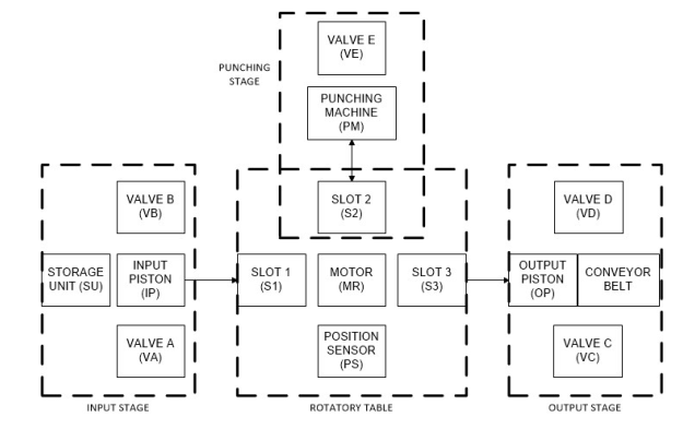Figure 1: AMS Topology

A(q23) → Θ(m10)	(20)
A(q25) → Θ(m8)	(21)

Using Lemma 22, the induced system for the BCs from Eqs. 18-21 is presented in Eq. system 22 consisting of a linear system of 8 inequalities. Employing the method proposed in section 3 (Theorem 23 and corollary 24) Eqs. 18-21 are transformed into a set of 4 linear inequalities shown in Eq. system 23.

q27 − m3 ≤ 0 q27 − m13 ≤ 0 q27 − m11 ≤ 0

                                  q27 − m−6m−2m8 ≤ 0                           (22)

q19 ≤ 0 q19 − m15 ≤ 0 q23 − m10 ≤ 0

q25 − m8 ≤ 0

7q27 − 2m3 − 2m13 − 2m11 − m6 − m8 ≤ 0

2q19 ⁻ m−2m⁻10m≤150^{≤ 0}     (23) q23

q25 − m8 ≤ 0

Using Eq. system 23 with the IBCD method, a PN supervisor is designed. The matrix L is defined in Eq. system 24. Using the equation D_c = −L ∗ D_p incidence matrix D_c of the supervisor is calculated, ans it is shown in Eq. system 25. Four self-looped arcs are added, one for each BC, connecting the monitor place with the corresponding controllable transition. The weight of each arc is the corresponding coefficient for the transition in the set of induced inequalities shown in Eq. system 23.The equation M_oc = −L ∗ M_o is used for calculating the initial marking vector M_oc of PN supervisor, shown in Eq. 26. Each monitor place is connected only to some transitions in the open loop model. Thus, each monitor place can be represented as a modular supervisor, using only the PN blocks connected to the monitor place. The resulting 4 modular PN supervisors are shown in Fig. 4.

4.3       Properness analysis

This subsection presents the analysis to show that the designed SCBC is in fact proper, i. e. the SUS is live, non-conflicting and controllable. For each BC, there are not 2 places belonging to the same PN block. Each PN block is a minimal S-invariant (see [11]).Therefore, there are not 2 places belonging to the same minimal S-invariant. Hence, by Proposition 29 the associated marking vectors for all the BCs are reachable. Now, by Proposition 30 in those markings the respective formulaes Φ are true. Since all transition of the BC are enabled in its respective associated reachable markings by Theorem 32 the SUS for every BC is live.

Now, by Theorem 33 the PN supervisor must not have any not live subnet in order to prove that the set of constraints is non-conflicting. However, the only not disjoint subnet of PN supervisor is concerned to transitions T₇ and T₈. From a quick analysis it is clear that this particular subnet is live. Hence, by 34 and Theorem 33 the SUS is live, i.e. the set of BCs is nonconflicting.

The set of constraints must be proven admissible. By Theorem 38, the set of constraints is proven admis-

sible since transitions T₂₇, T₁₇, T₂₁ and T₂₅ are controllable.

4.4 Ladder diagram implementation of supervisory controller

A PN can be translate into a ladder diagram for its implementation in a control device (e.g. a PLC). The general procedure for the translation of PN into ladder diagram is explained in [14]. Every place has a corresponding register in the ladder diagram. Every transition has a corresponding contact and its execution generates the change of the contact state.

The following rules are an adaptation of the translation procedure developed in [14]. Let T_a be a transition in the supervisor PN. Let P_a be an output place of T_a, connected by an arc with weight na. Let P_b be an input place of T_a, connected by an arc with weight nb.

• Each transition T_a is represented as a contact in a ladder segment.
• If P_a is 1−bounded, then it is represented by a coil with a set function. If P_a is not 1−bounded, then it is represented by an add block, adding na tokens to P_a.
• If P_b is 1−bounded, then it is represented by a coil with a reset function. Also,a normally open contact is associated to P_b in the segment.
• If P_b is not 1−bounded, then it is represented by a subtract block, subtracting nb tokens to P_b. Also, a comparison contact is associated to P_b, with the rule, greater or equal than nb.
• If P_a = P_b (self-loop), then the number of tokens holds. Thus, there are not output blocks associated to P_a in the segment.

The resulting ladder diagram for the SCBC is composed by 28 segments, one for each transition of the AMS model. A part of this ladder diagram is shown in Fig. 4.4. Each segment contains the conditions to enable the corresponding transition. For example, monitor place C1 must have at least 7 tokens for enabling transition T27. The number 7 is the coefficient corresponding to transition T₂₇ in the Eq. system 23. Moreover, in the Fig. 4 the weight of the bidireccional arc from monitor place C1 to transition t₂₇ is 7. Monitor place C4 must have a token for enabling transition T25.

Component Discrete Value Place Event Transition Type Storage Unit (SU) No piece in storage P1 Piece arrives to storage T1 uc   Piece in storage P2 Piece leaves from storage T2 uc Input piston (IP) Input piston in P3 Activate input piston T3 uc   Input piston out P4 Retract input piston T4 uc Slot 1 (S1) No piece in slot 1 P5 Piece arrives to slot 1 T5 uc   Piece in slot 1 P6 Piece leaves from slot 1 T6 uc Slot 2 (S2) No piece in slot 2 P7 Piece arrives to slot 2 T7 uc   Piece in slot 2 P8 Piece leaves from slot 2 T8 uc Slot 3 (S3) No piece in slot 3 P9 Piece arrives to slot 3 T9 uc   Piece in slot 3 P10 Piece leaves from slot 3 T10 uc Punching machine (PM) Machine withdrawn P11 Activate punching machine T11 uc   Machine active P12 Retract punching machine T12 uc Output piston Output piston in P13 Activate output piston T13 uc   Output piston out P14 Retract output piston T14 uc Position sensor of Loading position P15 Arriving to loading position T15 uc rotatory table (PS) Not in loading position P16 Leaving from loading position T16 uc Valve A (VA) Valve A closed P17 Open valve A T17 c retract input piston Valve A open P18 Close valve A T18 c Valve B (VB) Valve B closed P19 Open valve B T19 c activate input piston Valve B open P20 Close valve B T20 c Valve C (VC) Valve C closed P21 Open valve C T21 c retract output piston Valve C open P22 Close valve C T22 c Valve D (VD) Valve D closed P23 Open valve D T23 c activate output piston Valve D open P24 Close valve D T24 c Valve E (VE) activate Valve E closed P25 Open valve E T25 c punching machine Valve E open P26 Close valve E T26 c Rotatable Motor (MR) Motor off P27 Turn on motor T27 c   Motor on P28 Turn off motor T28 c Figure 3: Elementary components, discrete values and events of AMS with the corresponding places and tran-

sitions assignment (uc, uncontrollable; c, controllable)

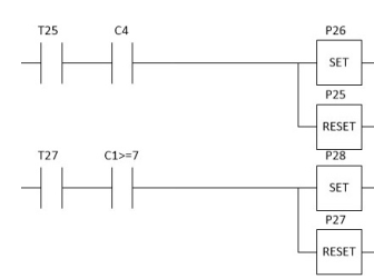Figure 4.4 Ladder diagram

5 Conclusions

The approach presented in this work reduces the number of monitor places needed to impose a set of constraints in a AMS. In the case study, the safety specification were successfully imposed in the system behavior using 4 monitor places, showing the exact same results that using the classical approach with 8 monitor places.

The incidence matrix of a discrete event system modeled as a PN usually has a lot of zero entries. The proposed approach reduces the dimension of Matrix L of the IBCD method, avoiding unnecessary by-zero multiplications giving a computational numerical advantage.

In the context of discrete event system the state expansion leads to complicated and unreadable graphs representations, such as Finite State Machines. The use of PN gives a more compact representation of the system, but it is still possible to find very complex graphs representations when a SC is design.

It has been proposed a synthesis method for a class of BC with a restricted syntax. Giving rise to a minimal PN SC. This increases the variety that can be considered in the synthesis (i.e. forbidden states) using a solid and mathematically established procedure.

The safety specifications ensure a behavior that forbids to any unwanted situation occurs in the system. The implementation was made using techniques previously proposed. The resulting implementation is compact and is a more usable approach for manufacturing systems.

Appendix A: Proof of Theorem 23

Proposition 39 Let x, y₁, y₂ be integer variables with

1. Nuñez et al. / Advances in Science, Technology and Engineering Systems Journal Vol. 2, No. 4, 32-43 (2017)

 0    0 L1 =  0     0	0 −1 0 0	−2 0 0 0	0 0 0 0	0 0 0 0	−1 0 0 0	0 0 0 0	−1 0 0 −1	0 0 0 0	0 0 −1 0	−2 0 0 0	0 0 0 0	−2     0      0 0       0     −1 0       0      0 0       0      0 h L =      L1	0   0   0  0  i 0	(24)
 0    1 Dc1 =  0     0	0 −1 0 0	−2 0 0 0	2 0 0 0	1 0 0 0	−1 0 0 0	1 0 0 1	−1 0 0 −1	0 0 1 0	0 0 −1 0	−2 0 0 0	2 0 0 0	−2       2      0 0         0        −1 0         0      0 0         0      0 h Dc =              Dc1	0      1      0  0  i 0	(25)
				MocT = h 6			1	0	i 0					(26)

Figure 4: a) Modular supervisor for monitor place C1. b) Modular supervisor for monitor place C2. c) Modular supervisor for monitor place C3. d) Modular supervisor for monitor place C4

domain {0,1}. The solution set for inequality

                                    (x − y₁)+(x − y₂) ≤ 0                             (27)

is the same solution set for the system

x −− yy1₂ ≤≤ 00          (28) x

Proof. The solution set of an inequalities system agrees to the intersection of each inequality solution set. Let predicate 29 be associated to system 28 and predicate 30 be associated to ineq. 27.

P [(x − y1 ≤ 0)] ∧ P [(x − y2 ≤ 0)]	(29)
P [(x − y1)+(x − y2) ≤ 0]	(30)

Table 39 shows that both expressions are equivalent.

Table tab:T1 Truth table for Proposition 39 x y₁ y₂ Eq. (29) Eq. (30)

• 0 0 T              T

                     0      0       1             T                   T

                     0      1       0             T                   T

• 1 1 T              T 1          0              0              F              F
• 0 1 F              F
• 1 0 F              F 1           1              1              T              T

Lemma 40 Let x, y₁, …y_n be integer variables with domain {0,1} and n ≥ 2. Y = y₁ + y₂ ···y_n. Let R =

{(x,Y)|x = {0,1},Y = {0,1,··· ,n}} be the constrained domain. Let Σ ⊂ R the solution set for the inequalities sys-

x − y₁ ≤ 0 x − y₂ ≤ 0tem

… x − yn ≤ 0 Then Σ is the solution set for the inequality	(31)
(x − y1)+(x − y2)+ ··· +(x − yn) ≤ 0 or in a compact form	(32)
nx − Y ≤ 0	(33)

Proof. (By mathematical induction) Let the base case be Proposition 39. The induction hypothesis of the inductive step is the Lemma statement. Therefore, it must be proved that the solution set of ineq. 34 and system 35 is the same.

            (x − y₁)+(x − y₂)+ ··· +(x − y_s)+(x − y_s+1) ≤ 0             (34)

x − y₁ ≤ 0 x − y₂ ≤ 0

^...         (35) x − y_s ≤ 0

x − y_s+1 ≤ 0

Ineq. 34 holds if and only if

                                           x − y_s+1 ≤ 0                                    (36)

holds and

                         (x − y₁)+(x − y₂)+ ··· +(x − y_s) ≤ 0                  (37)

also holds. This is derived from the fact that x can only take values 0 and 1. If Σ is the solution set for ineqs. 36 and 37, then σ is the solution set for 34. By induction hypothesis, if ineq. 37 holds, then system x − y₁ ≤ 0 x − y₂ ≤ 0

…

x − y_s ≤ 0

also holds. Therefore, Σ is the set solution for system 35 and it is proven that Σ is solution for 34 and 35.

Lemma 41 Let X, y₁, y₂, ··· , y_n, z₁, z₂, ··· z_m be integer variables with domain {0,1}. Let Y = y₁ + y₂ + ···y_n, Z = z₁ + z₂ + ···z_m. Let R = {(X,Y,Z)|X = {0,1},Y = {0,1,···n},Z = {0,1,···m}} be the constrained domain.

Let Σ ⊂ R the solution set for the inequality

m(nX − Y)+(x − Z) ≤ 0 Then Σ is also the solution set for the system X − y1 ≤ 0 X − y2 ≤ 0	(38)
…	(39)

X − y_n ≤ 0

X − Z ≤ 0

Proof. The proof consists of two steps. First the inequality 38 is derived from a geometrical perspective. Then, it is proven that if Σ is solution for eq. 38, then it is also solution for system 39. By Lemma 40, the first n inequalities are equivalent to ineq. 33, therefore system 39 becomes

nX ⁻ Y ^≤ 0

                                                 − Z ≤ 0                                     (40)

X

From a geometric perspective, both inequalities in system 40 have a corresponding plane in a tree dimensional space (X,Y,Z). The solution set for each inequality is constructed with the points contained in domain R and bounded above by the corresponding plane, thus the solution set for system 39 is constructed with the points contained in domain R and bounded above for the intersection of both corresponding planes. Therefore, there is a plane such that contains the intersection of both planes and bounds above all the points contained in domain R and the solution set of system 40. The intersection of these planes is a line containing the points (0,0,0) and (1,n,1). In order to describe a plane equation, an orthogonal vector to the plane is required, and for its calculation a third point is obtained by convenience, (_(mn^m₊₁₎,1,0). the orthogonal vector is obtained by calculating the cross product of two vectors in the plane, for simplicity, v₁ =< 1,n,1 > and v₂ =< m,mn+1,0 >.

Figure 41 Solution plane

                  i              j            k

        v           .

m

The plane equation is (mn+1)X − mY − Z = 0. Thus, the solution set for (mn + 1)X − mY − Z ≤ 0 is the same of system 39. Fig. 1. shows the plane and the constrained domain R. Now it is proven that solution set Σ for ineq. 38 is the same for system 39. System 39 holds for X = 0. If X , 0, because of the domain constraint, then X = 1. If X = 1, 39 holds for y_i ≥ 1 and Z ≥ 1, then Y ≥ n. Again because of the domain constraint, Y = n. Hence the set Σ that holds for expression 41 is the solution set for system 39.

                              (x = 0) ∨ [(Y = n) ∧ (Z ≥ 1)]                      (41)

x = 0           Y = n       Z ≥ 1                (x = 0) ∨ [(Y = n) ∧ (Z ≥ 1)]

       F             F              F                                   F

       F             F              T                                  F

F T F F F T T T T F F T

       T             F              T                                  T

       T             T              F                                   T

       T             T              T                                  T

Table 41 Truth table of equation 41

x = 0            Y = n       Z ≥ 1                 P [(mn+1)x − mY − Z ≤ 0]

        F             F              F                                  F

        F             F              T                                 F

F T F F F T T T T F F T

        T             F              T                                 T

        T             T              F                                  T

        T             T              T                                 T

Table 41 Truth table of equation 38

The truth table of expression 41 is shown in Table 41. Using definition 20, the truth table for predicate variable for ineq. 38 P ((mn+1)x−mY −Z ≤ 0) is showed in Table 41. It can be seen that there is a logical equivalence between expression 41 and ineq. 38 associated predicate.

Constraint 9 can be transformed to a system with n+1 inequalities, as established in Lemma 22

qa − mk₁ ≤ 0 qa − mk₂ ≤ 0

                                                   ^...                                            (42)

qa − mk_n ≤ 0

qa − [mj1 +mj2 + ··· +mjm] ≤ 0

By Lemma 40, the first n inequalities are equivalent to inequality

nqa − [mk1 +mk2 + ··· +mkn] ≤ 0 Hence the new system	(43)
nqa − mK ≤ 0 −        ≤	(44)

                                          q_a       m_J         0

Variables q_a, m_K, m_J satisfy conditions of Lemma

41. Therefore inequality

m[nq_a − m_K]+[q_a − m_J] ≤ 0 (45) shares the same solution set with system 44 and, henceforth, with system 42.

1. A. Sanchez, F. Jaimes, E. Aranda-Bricaire, E. Hernandez, A. Nava, Synthesis of product driven coordination controllers for a class of discrete event manufacturing systems, Robotics and Computer Integrated Manufacturing 26 (2010) 361 – 369.
2. C. Yang, W. Shen, T. Lin, X. Wang, A hybrid framework for integrating multiple manufacturing clouds, The International Journal of Advanced Manufacturing Technology 86 (1) (2016) 895–911. doi:10.1007/s00170-015-8177-9. URL http://dx.doi.org/10.1007/s00170-015-8177-9
3. W. Wonham, Supervisory Control of Discrete-Event Systems. Systems Control Group, ECE Dept, University of Toronto, http://www.control.toronto.edu/DES (2013).
4. M. V. Iordache, P. J. Antsaklis, Concurrent program synthesis based on supervisory control, in: American Control Conference (ACC), 2010, 2010, pp. 3378 – 3383.
5. D. Coman, A. Ionescu, M. Florescu, Manufacturing system modeling using petri nets, in: International Conference on Economic Engineering and Manufacturing Systems Brasov, November 2009, Vol. 10, 2009, pp. 207–212.
6. J. O. Moody, P. J. Antsaklis, Supervisory Control of Discrete Event System Using Petri Nets, Kluwer Academic Publishers, 1998.
7. A. Giua, F. DiCesare, M. Silva, Generalized mutual exclusion contraints on nets with uncontrollable transitions, in: IEEE International Conference on Systems, Man, and Cybernetics, Vol. 2, 1992, pp. 974–979.
8. E. Yamalidou, J. Kantor, Modeling and optimal control of discrete-event chemical processes using petri nets, Computers and Chemical Engineering 15 (7) (1991) 503 – 519.
9. A. Dideban, H. Alla, Reduction of constraints for controller synthesis based on safe petri nets, Automatica, International Federation of Automatic Control 44 (7) (2008) 1697–1706.
10. C. Baier, J.-P. Katoen, Principles of Model Checking, The MIT Press, 2008.
11. J. Desel, J. Esparza, Free Choice Petri Nets, Cambridge University Press, 2005.
12. A. Núñez, A. Sanchez, Supervisory control based on behavioral constraints using a class of linear inequalities, IFAC-PapersOnLine 48 (3) (2015) 2189 – 2194. doi: http://dx.doi.org/10. 1016/j.ifacol.2015.06.413. URL http://www.sciencedirect.com/science/article/pii/S2405896315006527
13. M. V. Iordache, P. J. Antsaklis, Supervisory Control of Concurrent Systems A Petri Net Structural Aproach, Birkhauser, 2006.
14. G. Gelen, M. Uzam, The synthesis and {PLC} implementation of hybrid modular supervisors for real time control of an experimental manufacturing system, Journal of Manufacturing Systems 33 (4) (2014) 535 – 550. doi: http://dx.doi.org/10.1016/j.jmsy.2014.04.008. URL http://www.sciencedirect.com/ science/article/pii/S0278612514000466

(Click to view)

(Click to view)