1      Introduction

Before their use as combustible in industrial furnaces for energy production, materials have to be tested at a laboratory scale. Their physical and chemical properties have to be determined, together with their energy power. Very small amounts of such materials (few milligrams) are tested in a thermobalance where the surrounding gas is injected and for which the evolution of the temperature, from ambient temperature to 900 ^◦C generally under a low heating ramp, is controlled with high accuracy. This thermobalance measures the remaining mass with a high precision along the experiment. During a thermogravimetric analysis, the chemical products which are emitted may also be analyzed. Figure 1 presents an example of mass loss and mass loss rate curves during the combustion process of a Cameroonian woody biomass in a thermobalance.

Two peaks appear on the mass loss rate curve (red), with shoulders on both sides of the main peak, all occurring in successive temperature ranges and corresponding to more intensive emissions of chemical

species. The thermal degradation is indeed obtained through a progressive destruction of the material structure under the influence of the gas (here synthetic air) which is injected and of course of the increasing temperature. While different molecules are released, the carbon structure is progressively destroyed. Under non-oxidative atmospheres, the mass associated to this carbon structure is almost preserved, while under air, this carbon structure is totally destroyed and removed. Only ash containing minerals remain at the end of the experiment. It is important to notice that even under (synthetic) air, such experiments do not lead, up to very rare and limited occurrences, to the presence of flames inside the thermobalance.

When modeling the thermal degradation of combustible materials in a thermobalance, as the diameter of the pan is few millimeters long, the space variables may be omitted and one can reasonably consider the evolution of the mass with respect to only the time parameter. All biomass are composed of three constituents: hemicellulose, cellulose and lignin, plus the carbon structure (and ash, moisture…) which are

known to degrade in different but superimposing temperature ranges. The relative fractions of these constituents depend on the material and the bonds between them influence the thermal degradation of the material.

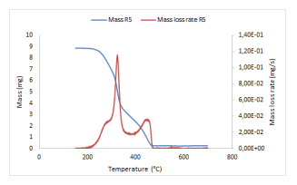Figure 1: Mass and mass loss rate curves for a Cameroonian wood residue, temperature ramp of 5 ^◦C/min, under synthetic air.

Based on this assumption and observation, different models have already been proposed for a representation of the thermal degradation in a thermobalance of a material considered either as global or as the sum of different constituents which are being degraded in an almost independent way, as their chains are intricate with the carbon structure.

More complex models are now being proposed which are based on balances which are written: masses of the different chemical species which are emitted during the experiments, momentum, energy. Of course, such complex models involve many equations and one usually needs a dedicated software for their numerical resolution.

In the different available models, constants have to be determined from the experimental results. They are called kinetic parameters and they are characteristics of the material and of the experimental conditions. The resolution of a model has thus to be coupled with an optimization procedure which determines the optimal set of kinetic parameters.

The purpose of this talk is to present a review of such models, from the simplest ones to the more complicated ones.

2           Kinetic modeling through a differential isoconversional method

The differential isoconversional method determines the values of the kinetic parameters associated to the thermal degradation of a material performed in a thermobalance, considering the material as global. It starts with the ordinary differential equation

see [1], which expresses the variations versus time of the extent of conversion α taken as

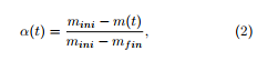where m_ini (resp. m(t), m_fin) is the initial (resp. remaining at time t, final) mass of the sample. In (1), k(T) is given an Arrhenius expression k(T) = Aexp(−Ea/RT), T being the temperature expressed in Kelvin (K) and which evolves with respect to the time parameter t from the ambient temperature T₀ with a constant rate a: T(t) = at + T₀. Here A is the frequency factor and Ea is the activation energy associated to the thermal degradation process of the material under consideration. Many functions f(α) have been proposed, starting from Mampel’s first-order function f₁ (α) = 1−α. Another one is the 3D diffusion function f₃ (α) = 1.5(1−α)^2/3/(1−(1−α)^1/3). The unique ordinary differential equation (1) is supposed to simulate the overall thermal degradation process.

It is impossible to solve the equation (1) in an explicit way. Many researchers already proposed different approximations of the right-hand side of (1) in order to obtain approximate solutions to this simple ordinary differential equation.

Instead of solving this equation, the differential isoconversional method consists to find the values of the kinetic parameters A and Ea, dividing (1) by f(α(t)) and taking the logarithm of the two members of (1). This leads to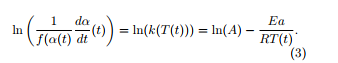

The values of the left-hand side of the preceding equality (3) are plotted for successive values of the extent of conversion α and for different temperature ramps (at least three), in terms of 1/T. The ICTAC recommendations suggest to take values of the extent of conversion α with steps not larger than 0.05, see [1]. The parameters of the straight lines which are plotted for different values of the extent of conversion using a linear regression lead to the determination of ln(A) (hence of A) and of Ea. Figure 2 presents such an

example

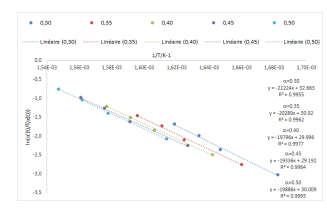Figure 2: Straight lines for successive values of the extent of conversion and for four temperature ramps.

One obtains values of the kinetic parameters A and Ea which are global for the material but which depend on the extent of conversion α.

	Mampel’s function
α	A (1/s)             Ea (kJ/mol)
0.05	2.2	23.0
0.10	3.5 × 1011	134.7
0.15	1.2 × 109	110.0
0.20	7.0 × 107	97.8
0.25	1.7 × 107	92.6
…	…	…
	3D diffusion function
α	A (1/s)             Ea (kJ/mol)

                     0.05                   3.2                      23.0

                     0.10      5.4 × 10¹¹                               134.7

                     0.15       1.3 × 10⁹                               110.0

                     0.20       1.3 × 10⁸                                  97.7

                     0.25       3.3 × 10⁷                                  92.5

                        …                …                         …

What can be done with such lists of values of the kinetic parameters? First, take mean values and standard deviations in order to obtain a unique couple of kinetic parameters valid for the material. But large variations of the kinetic parameters may be observed through the different lines. For small or large values of α, the precision of the experimental measurements is not really ensured, as very low amounts of the material are being degraded. But even when removing these lines, large variations may still be observed. A second tool consists to propose a reconstruction process which solves (1) stepwise, according to the time intervals associated to the stepwise changes of the extent of conversion. On two examples proposed in the GRE lab, this reconstruction process led to poor simulations. Probably because the isoconversional method uses logarithms.

This differential isoconversional method gives global values of the kinetic parameters for the material, but which change according to the extent of conversion, hence of the time (or temperature) parameter.

3                   Kinetic modeling through the EIPR model

3.1         Description of the model

The EIPR model superimposes the thermal degradations of three or four constituents of the material (in the case of a biomass: the H,C,L constituents of the sample, plus its char under an oxidative atmosphere), whose masses are supposed to evolve in an almost independent way. It leads to a unique set of kinetic parameters for each constituent of the sample. The initial mass m_ini of the sample is decomposed as m_ini = m(0)+m_ash +m_hum, where m(0) (resp. m_ash, m_hum) is the mass of volatiles which will be emitted and of char which will be produced (resp. ashes, moisture) in the sample. At time t, the remaining mass m(t) of the sample which can produce volatiles and char is given by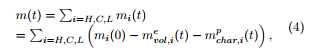

where m_i(t) is the mass of volatiles and of char contained in the constituent i (i = H,C,L) of the sample at time t, m_i(0) is the initial mass of the constituent i, which may be computed as a fraction of the overall mass of the sample: m_i(0) = c_im(0) (with c_H+c_C+c_L = 1), m^e_vol,i(t) is the mass of volatiles emitted by the constituent i of the sample (i = H,C,L), at time t and m^p_char,i(t) is the mass of char produced from the constituent i of the sample (i = H,C,L), at time t. The fraction coefficients c_i (i = H,C,L) for hemicellulose, cellulose and lignin have to be determined, which is not always an easy task. Chemical protocols have been defined for the determination of these fraction coefficients, but they currently lead to quite large uncertainties.

Under a non-oxidative atmosphere, only the volatiles are emitted during the thermal degradation of the material. Assuming first-order reactions for each constituent, the mass of volatiles emitted from the constituent i (i = H,C,L) evolves with respect to the time parameter according to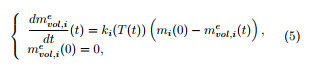

where T(t) is the temperature at time t in the sample (expressed in K) and which evolves with respect to the time parameter t from the ambient temperature T₀

with a constant rate a: T(t) = at + T₀. This leads to a non-coupled system of three equations, which can be compared to (1), in the case of Mampel’s function.

In (5), the kinetic constant k_i(T(t)) obeys an Arrhenius law: k_i(T) = A_i exp(−Ea_i/RT), where A_i (resp. Ea_i) is the frequency factor (resp. the activation energy) for the constituent i.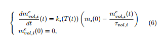

Under an oxidative atmosphere, the material looses its volatiles and its char is also consumed. For each constituent, the mass of volatiles emitted is supposed to be proportional to the mass of char produced, that is

,

with τvol,i + τchar,i = 1, τvol,i (resp. τchar,i) being the fraction of volatiles (resp. char) contained in the constituent i at time t. The fractions τ_vol,i of volatiles in H,C,L are specific to each material. The mass of volatiles emitted from the constituent i (i = H,C,L) here evolves with respect to the time parameter according to

Under an oxidative atmosphere, the mass of char remaining at time t in the constituent i of the sample at time t can be decomposed as m_char,i(t) = m^p_char,i(t) − m^c_char,i(t), where m^c_char,i(t) represents the mass of char consumed at time t among that ( )) which is produced from the constituent i of the sample (i = H,C,L). The mass of char is supposed to evolve with respect to the time parameter t according to a firstorder equation, as for the volatiles, but written as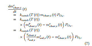

for i = H,C,L, where the kinetic constant k_comb (T) also obeys an Arrhenius law:

and where P_O2 is the oxygen pressure which is constant during the experiment (P_O2 = 2.026 × 10⁴ Pa).

Under an oxidative atmosphere, the coupled system of six ordinary differential equations has to be solved, with zero initial conditions

The problems (5) or (8) are solved using a numerical software (for example Scilab version 6.0.0) with given initial guesses of the kinetic parameters. An error is built which has to be minimized in order to determine the optimal set of kinetic parameters (A_i,Ea_i), i = H,C,L, (plus (A_comb,Ea_comb) under an oxidative atmosphere). This error involves the differences between the experimental and the simulated mass loss rates taken at experimental measure times (t_j)_j=1,…,J regularly distributed along the time interval (0,t_max) of the experiment, for example according to

where the simulated mass loss rate taken at time t_j is given under a non-oxidative atmosphere as

and under an oxidative atmosphere as

) being the experimental mass loss rate at time t_j. Instead of taking all the experimental measure times, only around 150 of them are indeed selected, regularly distributed along the overall experiment duration t_max. This reduces in a significant way the computing times.

Figure 3 presents an example of the simulated mass loss rate curves obtained through the EIPR method applied to a product derived from wood (hydrolysis lignin, after a torrefaction process at 275 ^◦C), where four (H,C,L+char) constituents are considered, because of the presence of two successive but ”connected” peaks. The mass loss rate curve associated to each constituent has been represented together with the sum (in blue) of these four partial curves. This blue curve is supposed to represent the experimental mass loss rate curve of the material (not represented on the figure).

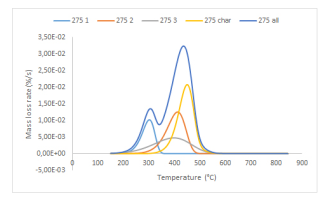Figure 3: Simulation of the thermal degradation of hydrolysis lignin torrefied at 275 ^◦C under air.

For this material, the optimal values of the kinetic parameters (A in 1/s) and Ea in J/mol) are obtained through the EIPR model as:

A1	9000000	A3	1.3
Ea1	110000	Ea3	47000
A2	110000	Acomb	10000000
Ea2	105000	Eacomb	135000

with the following values of the fractions of the three constituents and of the volatile fractions

c1	0.3	τvol,1	0.5
c2	0.3	τvol,2	0.9
c3	0.4	τvol,3	0.5

The maximal difference between the experimental and simulated mass loss rate curves is equal to 0.008 %/s, which has to be compared to the maximal mass loss rate curve, round 0.032 %/s.

3.2         Choice of the reaction function

In the above-indicated presentation of the EIPR model, a first-order reaction function has been used. Different functions may also be introduced, like in the differential isoconversional method, especially when the firstorder one does not lead to very good simulations of the thermal degradation of the material. For example, in the case of cotton residue, a unique peak is observed, as cotton is mainly composed of cellulose (more than 92%). But this peak is very narrow, as shown in Figure4.

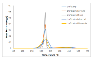Figure 4: Simulations through the EIPR model with different functions of the thermal degradation under air of cotton residue.

Different functions have been tested for the simulation of the thermal degradation of this cotton sample:

• the classical first-order function: f (α) = 1 − α;
• an Avrami-Erofeev reaction function: f (α) = 4(1 − α)(−ln(1 − α))^3/4;
• the Prout-Tompkins reaction function: f (α) = α(1 − α);
• a chain scission function.

The different functions which have been tested do not simulate in an appropriate way the very narrow devolatilization peak, see [7] for more details. Other reaction functions are available which should be tested.

In the EIPR model, the kinetic parameters are global but for each constituent of the material and they do not depend on the time parameter. The EIPR model has been tested at GRE lab for different materials, see [2] and [3] for example. Reference articles for the simulation of the thermal degradation of lignocellulosic materials with independent reactions are [4] and [5], among others. The independent decomposition of the three constituents of a lignocellulosic material is questionable. The interactions between the three constituents of a lignocellulosic material have recently been analyzed in [6].

3.3         Influence of the temperature ramp

It has been observed by several authors and for a long time that the temperature ramp influences the thermal degradation of a material. Shifts to higher temperatures indeed appear in the mass loss rate curves, which increase with the temperature ramp, see Figure 5 again in the case of the cotton residue.

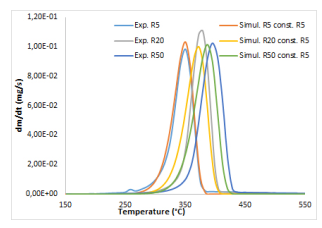Figure 5: Influence of the temperature ramp on the thermal degradation of cotton residue under nitrogen and on the simulation through the EIPR model.

The simulations through the EIPR model which lead to a quite perfect superimposition of the mass loss rate curves at 5 ^◦C/min fail at higher temperature ramps. This may be the consequence of diffusional limitations which occur in the material and which increase with the temperature ramp. In Figure 5, the mass loss rate curves have been transformed (multiplication by a fixed coefficient) in order to reach almost the same maximal value.

In [7], a heat transfer model has been proposed which brings corrections to the temperature really acting in the material. The temperature is supposed to evolve in the sample according to the classical heat transfer equation

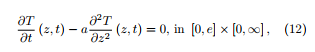where e is the thickness of the cotton sample put in the crucible of the thermobalance and the thermal diffusibility coefficient a is given through with:

• λ thermal conductivity of cotton, approximately equal to 0.038 W/mK,
• ρ density of cotton, approximately equal to 40 kg/m³,
• c specific heat coefficient of cotton, approximately equal to 1.725 kJ/kg.

Because of the structure of the TA Q600 thermobalance, the boundary condition

!

is considered at z = 0 (upper surface of the sample in contact with the surrounding heated atmosphere). In this boundary condition, h (resp. ε, σ) is taken equal to 5 W/m²K (resp. 0.9, 5.67 × 10⁻⁸ W/m²K⁴) and T_g (t) means the temperature of the heated gas surrounding the cotton sample. The temperature T_g (t) is measured in the thermobalance by a thermocouple located just under the crucible. The boundary condition

is imposed on the mid-thickness (z = e/2, with e = 0.001 m) surface of the sample, thus considering a symmetry of the sample layer with respect to its midthickness

The temperature T starts at t = 0 from the room temperature: T (z,0) = 20 ^◦C= 293.15 K.

The above heat transfer problem is solved through an implicit finite difference method with dt = 8950/896 = 9.99 s and dz = (e/2)/100 = 5.0 × 10⁻⁶ m, using the numerical software Scilab.

When solving this heat transfer model, typical curves representing the difference diff (t) between the measured temperature T_g (t) of the surrounding gas and the mean value (T (0,t) + T (e/2,t))/2 of the computed temperatures at the upper surface (z = 0) and at the mid-thickness (z = e/2) of the bed are given in Figure 6 for temperature ramps of 5, 20 and 50 ^◦C/min.

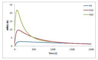Figure    6:      Differences   between   the      temperature

T_g                               of the surrounding gas and the mean value

(T (0,t) + T (e/2,t))/2 inside the sample, for temperature ramps of, 5, 20 and 50 ^◦C/min.

The difference diff (t) first increases and reaches its maximal value at 22 ^◦C (resp. 10 ^◦C) for a temperature ramp of 50 ^◦C/min (resp. 20 ^◦C/min). The differences between the gas temperature and the solid temperature are really significant and, consequently, have to be taken into account in the determination of the kinetic parameters. In the model (5), T (t), which was initially taken as the measured gas temperature T_g (t), is replaced by the computed mean value (T (0,t) + T (e/2,t))/2. For example, considering a temperature ramp of 50 ^◦C/min, a quite perfect superimposition of the devolatilization peaks may be observed between the experimental and the simulated mass loss rate curves using the above computed values of the kinetic parameters for a temperature ramp of 5 ^◦C/min and considering the above-indicated mean value temperature in the sample instead of T_g (t), see Figure 7.

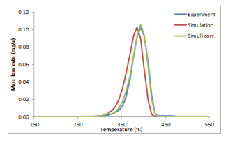Figure 7: Comparison between the experimental mass loss rate curve (blue) under nitrogen and under temperature ramp equal to 50 ^◦C/min, and the simulation with the values of the kinetic parameters obtained for a temperature ramp of 5 ^◦C/min without correction (red) or with the correction given by the mean value of the temperatures (green).

4           A simplified model accounting for the combustion of coal char particles in a drop tube furnace

4.1         Description of the experiment

Coal char particles are produced from coal particles through a pyrolysis process in a drop tube furnace. Volatiles are emitted from the coal particles and a swelling phenomenon occurs.

In a drop tube furnace, the temperature ramp is much higher than in a thermobalance: around 1500 K/s, against 10 K/min in a thermobalance. The drop tube furnace is 140 cm long and with an internal diameter of 5 cm. It is heated by resistances placed between its outer and inner envelopes. The reactor temperature is held fixed, here 1100, 1200 or 1300 ^◦C. This device simulates the behavior of industrial pulverized boilers.

For each combustion experiment, 2 mg of coal char particles are injected with an oxidative gas flow (88% N₂, 12% O₂, 40 l/hr) through a water cooled injector and entrained by a secondary nitrogen flow (360 l/hr) preheated at 900 ^◦C. During the fall in the drop tube furnace, the temperature of the coal char particle was continuously measured by a pyrometer placed at the bottom of the reactor and pointing vertically to the injection probe of the reactor.

The fall time of the coal char particle is very short:

around 1s.

4.2         Description of the model

As a simplifying hypothesis, the structure of the coal char particles may be considered as uniform at each time of the experiment. The temperature of the particle may also be supposed uniform inside the particle. Based on these hypotheses, a simplified model has been elaborated which intends to predict the temperature of the particle during its fall in the drop tube furnace.

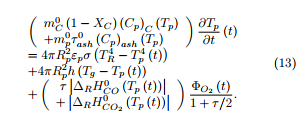
The energy balance during the heating up of a spherical char particle of fixed radius R_p is written as

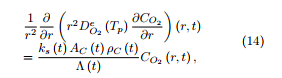
The equation for oxygen transport within the particle is written as

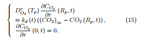
with the boundary conditions

The evolution of the conversion ratio X_C defined as X_C (t) = 1 − m_C (t)/m⁰_C is described through

the oxygen flux Φ_O2 entering the particle being defined through the expression

(CO2)∞

Φ_O2 (t)

.

The different coefficients which appear in equations (13)-(16) are known or are given known expressions.

The coefficient k_s (t) which appears in (14) is given an Arrhenius expression whose frequency factor and activation energy are deduced from experiments performed on the coal char particles in a thermobalance under an oxidative atmosphere and under a temperature ramp of 5 ^◦C/min, through the EIPR method described in the preceding section.

For the resolution of (13) and (16), an explicit Euler method has been applied (progression with respect to the time parameter). For the resolution of (14), a second-order finite difference method has been built, see [9] for the details of this method, which is slightly better than the classical finite element method but which does not require the introduction of complementary basis functions. Further, observe that the equation (14) is written in spherical coordinates. The equation may thus look as singular. But the boundary condition (15)₂ prevents from real singularity. The whole problem has been solved using a Fortran code.

The experimental and simulated temperature curves are gathered in Figure 8.

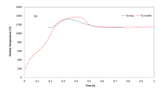Figure 8: Experimental and simulated temperature curves of a coal char particle injected in a drop tube furnace, with a regulation temperature of 1200 ^◦C.

The maximal difference between the experimental and simulated temperature particle is equal to 43 ^◦C in the interesting time range (0.2-0.8 s). This may seem high. But first the uncertainties of the temperature measurements in a drop tube furnace through a pyrometer are usually taken equal to 50 ^◦C, because of the important radiations from the reactor wall. Second, the accuracy of the pyrometer itself is given at 6 ^◦C. Finally, the relative difference is equal to 3%, which is largely acceptable.

Of course, this simplified model does not simulate the mass loss of the particle during its fall in the drop tube furnace, as it does not involve the evolutions of the chemical species during the combustion process.

A more sophisticated model is currently being developed in Mulhouse, which takes into account local variations of the structure of the particle during its fall in the drop tube furnace (pore opening, progressive destruction of the structure from the exterior of the particle).

5           More complex models accounting for the thermal degradation of materials

For the construction of such models, the chemical species which are emitted during the thermal degradation process have to be determined first. In [10], the authors give a long list of possible chemical reactions which may occur during biomass pyrolysis, together with the corresponding kinetic parameters which are given Arrhenius expressions. Then the balance equations are written, see [11], in the case of 3 (main) chemical reactions and 5 gas species, which lead to a coupled system of 8+7 equations (inside the particle and in a boundary layer around the particle).

5.1         Inside the spherical particle

• Conservation of each of the gaseous species (k =

1,…,5)

,

with l = 3.

• Total molar balance of gas mixture

.

• Energy balance equation

.

• Carbon mass balance

.

5.2         In a gas boundary layer

• Conservation of each of the gaseous species (k =

1,…,5)

.

• Total molar balance of gas mixture

.

• Energy balance equation

.

Initial and boundary conditions are added to this problem.

5.3         Other complex models

In [12], the authors introduce a simpler model, starting with the conservation law

,

in the case of a spherical particle, where ε is the porosity of the particle (which may evolve along the combustion process), ρ_g is the gas density, v its velocity and S_mass represent the mass sources due to a transfer to the gas phase. The balance of linear momentum is written using Darcy’s law as

,

where p is the pressure, µ the viscosity, k the permeability and C is a constant. The convection+diffuse transport of the gaseous species inside the particle is written as

,

where w_k,i,gas is a reaction term. Finally the energy conservation is written as

.

Appropriate boundary and initial conditions are also added.

In [13], the authors introduce quite similar balance equations but in a steady regime.

Of course, for the resolution of such coupled and complex systems of evolution equations, numerical codes have to be built or dedicated software have to be used. In their paper [11], the authors indicate that they used Comsol multiphysics software for the resolution of this problem.

Such complex models have not been solved in the GRE lab. Interested readers are referred to the indicated references and to the further references these limited references contain.

To our knowledge, existence and uniqueness results have never been proved for such coupled systems of evolution equations, although first they are based on balance equations and second they are certainly not ”singular” systems. A theoretical numerical resolution of such systems should be developed.

6           Conclusion

Throughout this presentation, different methods and models accounting for the thermal degradation of combustible materials under controlled temperature ramps and non-oxidative or oxidative atmospheres have been presented. Each method or model is based on hypotheses and presents limits, although the obtained simulation of the thermal degradation process is roughly acceptable. Mathematical analyses of the models should be done in order to also improve these simulations. The references listed below will help the interested readers for deeper understandings of these concrete experiments.

1. Vyazovkin, AK. Burnham, JM. Criado, LA. Perez- Maqueda, C. Popescu and N. Sbirrazuoli, “ICTAC Kinetics Committee recommendations for performing kinetic computations on thermal analysis data,” Therm. Acta 520, 1{ 19, 2011. http://doi.org/10.1016/j.tca.2011.03.034.
2. Valente, A. Brillard, C. Schonnenbeck and JF. Brilhac, “Investigation of grape marc combustion using thermogravimetric analysis. Kinetic modeling using an extended independent parallel reaction (EIPR),” Fuel Proces. Technol. 131, 297{303, 2015. http://dx.doi.org/10.1016/j.fuproc.2014.10.034.
3. Brillard, JF. Brilhac and M. Valente, “Modelization of the grape marc pyrolysis and combustion based on an extended independent parallel reaction and determination of the optimal kinetic constants,” Comp. Appl. Math. 36(1), 89-109, 2017. DOI 10.1007/s40314-015-0216-5.
4. Orfao, FJA. Antunes and JL. Figueiredo, “Pyrolysis kinetics of lignocellulosic materials – three independent reactions model,” Fuel 78, 349-358, 1999. PII: S0016- 2361(98)00156-2.
5. Damartzis, D. Vamvuka, S. Sfakiotakis and A. Zabaniotou, “Thermal degradation studies and kinetic modeling of cardoon (Cynara cardunculus) pyrolysis using thermogravimetric analysis (TGA),” Bioresour Technol. 102, 6230{6238, 2011. doi:10.1016/j.biortech.2011.02.060.
6. Yu, N. Paterson, J. Blamey and M. Millan, “Cellulose, xylan and lignin interactions during pyrolysis of lignocellulosic biomass,” Fuel 191, 140{149, 2017. doi:10.1016/j.fuel.2016.11.057.
7. Brillard, D. Habermacher and JF. Brilhac, “Thermal degradations of used cotton fabrics and of cellulose: kinetic and heat transfer modeling,” Cellulose 24(3), 1579-1595, 2017. DOI 10.1007/s10570-017-1200-6.
8. Gilot, A. Brillard, C. Schonnenbeck and JF. Brilhac, “A simpli_ed model accounting for the combustion of pulverized coal char particles in a drop tube furnace,” Energy Fuels, 31(10), 11391{11403, 2017. DOI: 10.1021/acs.energyfuels.7b01756.
9. Brillard, JF. Brilhac and P. Gilot, “A second-order _- nite di_erence method for the resolution of a boundary value problem associated to a modi_ed Poisson equation in spherical coordinates,” Appl. Math. Model. 49, 182{198, 2017. http://dx.doi.org/10.1016/j.apm.2017.04.034.
10. Anca-Couce and R. Scharler, “Modelling heat of reaction in biomass pyrolysis with detailed reaction schemes,” Fuel 206, 572{579, 2017. http://dx.doi.org/10.1016/j.fuel.2017.06.011.
11. Sadhukhan, P. Gupta and RK. Saha, “Modeling and experimental studies on single particle coal devolatilization and residual char combustion in uidized bed,” Fuel 90, 2132-2141, 2011. doi:10.1016/j.fuel.2011.02.009.
12. Peters, A. D_ziugys and R. Navakas, “A shrinking model for combustion/gasi_cation of char based on transport and reaction time scales,” Mechanika 18(2), 177-185, 2012.
13. Annamalai and IK. Puri, “Combustion science and engineering,” CRC Series in Computational Mechanics and Applied Analysis. CRC Press, Boca Raton, 2007.

(Click to view)

(Click to view)