1. Introduction

This paper provides an extension of the work presented in [1], which is based on a sensitivity analysis of handheld GPR measurements, comparing bi-static and multi-static system performance using singular value decomposition (SVD). The results obtained confirmed the conclusions of a previous study conducted by Watson [2], which states that multi-static systems achieve greater subsurface information, for a landmine detection application using full wave inversion (FWI). The study in [2] also conducted a 2D FWI to verify the superior performance of multi-static arrays over a bi-static configuration, for handheld GPR. It concludes that the size of the multi-static array, or number of antenna elements, is insignificant. Furthermore, the acquisition system under test was simplistic and radio propagation properties such as the antenna cross-coupling, radiation pattern and geometry are neglected. Additionally, only a flat, homogenous domain was simulated for the 2D FWI analysis.

Nevertheless, a 2D FWI study is insufficient, as the landmine detection domain is a 3D, heterogeneous domain and a 3D analysis is required to produce a more realistic evaluation of the performance of bi-static and multi-static handheld GPR systems for the demining challenge. Here, an empirical FWI numerical analysis is reported for a 3D domain, which considers a homogenous as well as a heterogeneous or cluttered domain, using a derivative-free optimization algorithm. The bi-static and multi-static system performance are evaluated by comparing the estimated subsurface parameters obtained in each case with synthetic GPR data parameters. All the radio propagation effects are included with simulated experiments conducted in the CST STUDIO SUITE 3D electromagnetic (EM) environment. Finally, a novel method to determine an improved initial parameter set for the GPR FWI optimization, that is closer to the global minimum, is proposed. This is achieved by generating a database of prior forward problem solutions. The database is used with each measured GPR data to determine the least L2 norm objective function, whose parameters are considered as the initial parameter set for the actual FWI optimization.

2. FWI for Multi-static Handheld GPR

2.1.  Gradient Based Method

     The GPR FWI problem for landmine detection may be posed as a regularised least squares (LSQ) non-linear optimisation problem given by [2]

where  is a vector of geometric and electrical parameters describing the ground, d is the GPR measured data,  is a forward model that returns the GPR measurement that would be made for a subsurface with parameter vector . The GPR inverse problem is ill-posed as arbitrarily large changes in  can have negligible effect on the error .  The regularisation term is required to control the size of components of  with little or no effects on GPR data.  The function  introduces a penalty based on the size of these components and is a way to introduce prior information.  For Tikhonov regularisation  and often  is chosen to be the identity matrix.  The regularisation or Tikhonov factor  is often adjusted dynamically during the iterative optimisation process to control convergence.  Optimisation is posed as a LSQ problem as the error functional uses the L2 norm.

The GPR forward model is non-linear and so (1) is often solved by iterative linearization.  Watson used an iterative, quasi Newton method called the limited memory Broyden-Fletcher-Goldfarb-Shannon (L-BFGS) nonlinear optimisation algorithm [3]. The solution requires a calculation of the gradients of the LSQ error function .  Due to the special form of the LSQ error function, these derivatives can be directly related to the derivatives of the forward model.

2.2.  Derivative-free Method

      The derivative-free method for solving the FWI problem is used because it is computationally expensive to estimate the derivatives required for derivative based methods.  Derivative-free methods require less computation per iteration and are suitable for a limited number of variables, but may require more iterations. A range of non-derivative nonlinear optimization algorithms may be used to solve the FWI optimisation problem when gradients do not exist or are expensive to compute. Local direct search methods may be used when there are a small number of variables and the objective function is computationally cheap to evaluate. The Nelder-Mead simplex algorithm [4] is the most cited, robust and efficient of local direct search methods. The algorithm fundamentally relies on an initial number of points that create a simplex i.e. a set of points spanning a volume in the variable dimensionality considered. The objective function is evaluated at the vertices of the simplex during each iteration to determine the highest objective value, which is used to redefine another vertex that produces a new simplex. Additional new points are produced by moving the vertex with the highest objective value through a series of transformations using the centroid of the associated simplex that include reflection, expansion, internal and external contractions [5]. These steps are iterated until convergence is achieved. Convergence can occur for non-smooth objective functions even when the second derivative of the function is unobtainable [6]. The Nelder Mead simplex algorithm may be applied to the FWI optimisation problem, to estimate the uncertainty in parameter sensitivity of the handheld GPR bi-static and multi-static systems. The Nelder Mead Simplex algorithm is embedded in the CST STUDIO SUITE environment and so the 3D GPR forward model may be integrated with the optimization process on the same platform.

3. Modelling and Simulation

3.1.  The GPR System Models and Experiments

The GPR system models are developed with linear antenna arrays positioned with dipoles at a fixed distance above the ground surface. The configurations are for a bi-static system, and multi-static system with two and four receive elements, driven in a single input multiple output (SIMO) sequence. The antennas are end-fed (coaxial) dipole antennas designed and optimised using the Antenna Magus software for a centre frequency of 2.5 GHz and frequency range of 1.75-3.25 GHz.  Assuming the same offset of 20 cm used by Watson, an antenna element spacing of 5 cm was used in all configurations. Antenna cross-coupling losses are significant, given this spacing which is less than a wavelength. The antennas are placed initially at a height of approximately 3.76 cm above the ground surface. The transmitting element is at the extreme left end of the array and the time series measured at each receive antenna are concatenated into a single data vector d.  The target object is placed under the centre of the array, based on the assumption that a metal detector (MD) has located a conducting part of the device.

      To reduce the computational cost, the ground size for this study is reduced to a 31 cm by 29 cm box with a depth of 9cm. The subsurface parameters are the relative permittivity and loss tangent . The target is a single AP mine which is modelled as a typical plastic cylinder with relative permittivity (typical US M14 mine).  The diameter and height are 7cm and 6cm respectively, closer to a Colombian military MN-MAP-1 mine [7].  The mine also contains a tetryl charge (US M14) with relative permittivity and an air void of free space relative permittivity of one. Instead of ABC boundary conditions (used by Watson), perfectly matched layer (PML) boundary conditions are applied on all faces of the box (ground) for all models in this study with added space above the antennas on the top of box to simulate the antenna to antenna and antenna to ground propagation. ABC boundary conditions have been studied longer and are generally easier to implement, but the PML region achieves less boundary reflections [8].

For a heterogeneous ground (cluttered domain), we introduce a rough surface to the flat ground (box) surface. The ground surface roughness height is modelled in the form of a Gaussian distribution [9]. Therefore, the box planar surface is modelled with depressions and protrusions to simulate a ground surface with a random height, assuming a Gaussian distribution, normally distributed white noise and a mean value of zero [10]. Additionally, subsurface clutter sources are modelled as several 3D rectangular blocks, grouped into two clusters, with each set having a different relative permittivity. One has a relative permittivity, and the other with a relative permittivity, . An example bi-static dipole system and target subspace is shown in Figure 1. A LSQ FWI regularised optimisation problem, as in (1), is the test problem. The goal value to be evaluated is the sum squared difference of the total simulated GPR data (time-series) and the total forward model data (time-series), which is given by .  Watson performed a similar study for dipole antennas in a simplified 2D, homogenous domain only. Here both 3D homogenous and heterogeneous domains are investigated for the FWI analysis.

The optimization is set to a maximum of 20 iterations, due to computational constraints. The hexahedral mesh used to produce

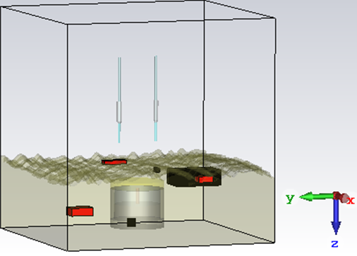Figure 1: Bi-static dipole system for a heterogeneous ground

synthetic GPR measurements is different from the mesh used in the forward model within the FWI objective function. This avoids the spuriously good results that can be the inverse crime artefact [11] due to using the same mesh for both operations.

The parameter vector for the synthetic GPR data for the homogenous ground is given by

where = relative permittivity of tetryl charge

= loss tangent

= relative permittivity of free space

= relative permittivity of plastic mine

= relative permittivity of dry sandy soil

Whereas the parameter vector for the synthetic GPR data for the heterogeneous ground is given by

where = relative permittivity of first clutter source

= relative permittivity of second clutter source

= relative permittivity of free space

= relative permittivity of plastic mine

= relative permittivity of dry sandy soil

The initial subsurface parameter vector for the homogenous ground FWI is given by

Whereas the initial vector for the heterogeneous ground FWI is given by

3.2.  FWI Numerical Analysis Results

To estimate the performance of the different antenna systems, we compare and consider the estimated parameter values approached by the FWI solutions for both models with their respective synthetic GPR data true parameter values. The error in the subsurface parameters for each system in the different ground conditions is estimated by determining the total sum squared difference between the GPR data vector parameters and the FWI solution vector parameters. The total estimated parameter errors are indicated in Tables 1 and 2 for the homogenous ground and heterogeneous ground respectively.

The 3D FWI data shows that for both ground domains, the conclusion that multi-static systems can achieve more subsurface information is achieved as the smallest subsurface error in both cases is recorded with a multi-static system. At this stage, we can confirm that the multi-static system performs better than the bi-static system in general. However, the subsurface parameter error is not monotonic for the number of antenna elements whereas it was found to be linear for a 2D FWI analysis. These results based on a 3D analysis are more realistic as the scattering on the soil surface and cylindrical mine introduce more degrees of freedom and complexity than a 2D numerical analysis.

For the homogeneous soil, the 4 receiver (RX) system FWI achieves a better performance than the two other systems though the difference between the bi-static system and 2 RX multi-static system is marginal. However, in the more realistic heterogeneous domain the 4 RX multi-static system yields the largest parameter uncertainty. The scattering and clutter signals are observed to be larger in the heterogeneous domain than the homogenous domain based on the larger subsurface parameter error and uncertainty figures that are estimated in the former. This is due to greater air-ground reflections from the rough ground surface and scattering from the buried clutter sources. In this case the clutter signal is much larger than the mine signal. Nevertheless, for both soils, particularly the heterogeneous soil, the parameterisation does not sufficiently describe the clutter and so the optimisation easily converges to the wrong solution.  Some method is required to reduce the effects of the clutter signal.  Therefore, better imaging with multi-static systems for a real GPR system and demining operation based on FWI is predicated on an optimised antenna design as well as clutter reduction.

Conversely, this analysis also shows that the multi-static system achieves only a small improvement over the bi-static system. A FWI optimization with actual GPR measurements or field evaluation data is expected to exhibit greater complexity and hence the improvement may only be marginal. This study has been limited to synthetic data and future studies may include further validation of the results obtained with the use of measured GPR data.

Table 1: Summary of GPR and FWI solution parameter values for homogenous ground

Subsurface Parameters	GPR Data Parameter Values	FWI Solution Estimated Parameter Values
		Bi-static	Multi-static (2RXs)	Multi-static (4RXs)
Charge relative permittivity	2.163	2.292	2.268	2.3
Loss tangent	0.0036	0.0026	0.0034	0.0069
Air void relative permittivity	1.0	1.49	1.5	1.45
Mine relative permittivity	2.8	3.069	3.185	3.032
Soil relative permittivity	2.53	2.2	2.2	2.6
Estimated parameter error	–	1.219	1.320	0.892

Table 2: Summary of GPR and FWI solution parameter values for heterogeneous ground

Subsurface Parameters	GPR Data Parameter Values	FWI Solution Estimated Parameter Values
		Bi-static	Multi-static (2RXs)	Multi-static (4RXs)
Charge relative permittivity	2.163	2.4	2.388	2.314
Clutter1 relative permittivity	3.75	2.25	2.25	2.25
Clutter2 relative permittivity	6.0	7.28	6.67	8.0
Loss tangent	0.0036	0.0058	0.0066	0.0068
Air void relative permittivity	1.0	1.35	1.29	1.39
Mine relative permittivity	2.8	3.04	2.96	3.16
Soil relative permittivity	2.53	2.27	2.33	2.2
Estimated parameter error	–	3.869	3.048	4.734

4. Improvement of the FWI Initial Parameter Set

The steepest descent and direct search methods for iterative nonlinear optimisation all require an initial parameter set which is updated iteratively according to the chosen method. The GPR FWI problem is also a local minimisation problem that is nonlinear as well as ill-posed. A good initial parameter set that is as close as possible to the true solution is desirable to ensure convergence to the global minimum and less computational expense. A more general approach would be to employ global optimization techniques prior to the local optimization. However, for the GPR problem this would be computationally prohibitive. We propose a compromise approach that involves solving the forward problem for several parameter sets within the bounded local domain or search space and using an L2 norm objective with the true solution or measured data, as the goal value. The forward model meshing or grid would be set to the lowest tolerance level as only a coarse analysis is required to avoid a high computational expense. A higher tolerance is set for the forward model grid for the actual optimization.

A database of the forward model solutions for a specific operation is generated and can be evaluated with data from each GPR measurement. The initial parameter vector for the FWI solution is chosen by interpolation from the database of parameter vectors and measured time-series. Hence a single database is generated during a single campaign but can be used repeatedly for GPR data from the same source environment or location. The database campaign could be done during the training phase of a demining operation prior to the actual clearance operation. The database can be generated for any chosen number of parameter combinations and sample space or bounded conditions. More forward model solutions would be expected to increase the probability of a better initial estimate of the parameter set.  For this experiment, the 4 RX dipole system GPR model for a heterogeneous domain is utilised. Eleven forward model solutions are generated by arbitrarily choosing eleven different parameter sets for values between a minimum and maximum bound. This yields a database of eleven sets of A-scan data and the L2 norm objective value of each of these data for any measured GPR is determined. The parameter set for the time-series (A-scan) that achieves the lowest objective function value would be considered as the closest to the true solution or global minimum and selected as the initial optimization parameter set. Figure 2 presents the objective function value for all eleven forward problem solutions.

      It can be determined from Figure 2 that the lowest objective function value is obtained at simulation run eight which corresponds to a value of 0.001708. The parameter set for this forward model measurement,  is given by

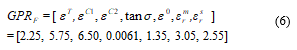Therefore, this parameter set given in (6) is selected as the initial parameter set for the iterative FWI solution, for the heterogeneous domain under test. The FWI optimization solution for this parameter set is then obtained for 20 iterations, due to computational constraints, and compared directly with the FWI solution for the initial parameter set in (3). The result is shown in Figure 3.

     The comparison of the FWI solution for the original initial parameter set and the one derived from the database generation (Figure 3) shows that the latter does not achieve an improvement in the accuracy of convergence as the absolute error is marginally less than the original solution. However, the result does show that the database generated initial parameter FWI solution is closer to the true solution. This could potentially lead to a more efficient optimization using a more powerful algorithm. Derivative based methods would benefit from this improvement and achieve convergence with less computational expense and fewer iterations as a local minimum would be realised more efficiently. The procedure achieves the primary goal of improving the initial parameter estimation or guess.  The CST integrated Nelder-Mead optimisation does not allow the user to specify the entire simplex and objective function values.  If this had been the case, the initial 10 iterations exploring the simplex could have been entirely avoided by selecting all the simplex points from the database. The performance of gradient based algorithms are expected to benefit from the database generated improved initial parameter set.

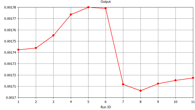Figure 2: Objective function values for eleven forward problem solutions

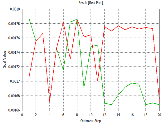Figure 3: FWI solution result for 4 RX dipole a. original initial parameter set (GREEN) versus database selected parameter set (RED)

5. Conclusion

An empirical study has been undertaken to compare 3D FWI imaging using multi-static and bi-static systems in homogeneous and heterogeneous media. The results verify the possibility of multi-static systems to achieve greater subsurface parameter sensitivity and hence reliability of target detection than bi-static systems. In 2D, all multi-static systems outperformed the bi-static systems. However, a more realistic 3D analysis shows that the improvement in performance with increasing numbers of antennas is not simple or monotonic due to cross-coupling and antenna patterns.  This underlines the need for optimisation of the antenna system configuration and size (number of elements), to achieve better performance than a bi-static system. Additionally, the effect of clutter significantly limits the accuracy of parameter estimation. Finally, a novel procedure has been proposed to determine the initial parameter vector for the FWI solution which yields an initial forward problem solution that is closer to the true GPR data solution. The procedure requires numerous forward problem solutions stored prior to a deeming campaign but has the potential to significantly reduce the computational expense of the FWI as well as the accuracy for an ideal local minimisation.

Conflict of Interest

The authors declare no conflict of interest.

Acknowledgment

The authors would like to acknowledge the Petroleum Technology Development Fund (PTDF), Abuja, Nigeria.

1. Sule, S.D. and Paulson, K.S., “A comparison of bistatic and multistatic handheld ground penetrating radar (GPR) antenna performance for landmine detection”, IEEE Radar Conference (RadarConf), 2017, pp. 1211-1215. DOI: 1109/RADAR.2017.7944389
2. Watson, F. and Lionheart, W., “SVD analysis of GPR full-wave inversion”, 15th International Conference on Ground Penetrating Radar (GPR), 2014, IEEE, pp. 484-490. DOI: 1109/ICGPR.2014.6970472
3. Nocedal, J. and Wright, S., Numerical optimization. Springer Science & Business Media, New York, 2006.
4. Nelder, J.A. and Mead, R., “A simplex method for function minimization”, The computer journal, 7(4), pp. 308-313, 1965. https://doi.org/10.1093/comjnl/7.4.308
5. Rios, L.M. and Sahinidis, N.V., “Derivative-free optimization: a review of algorithms and comparison of software implementations”, Journal of Global Optimization, pp. 1-47, 2013. doi:1007/s10898-012-9951-y
6. Mckinnon, K.I., “Convergence of the Nelder–Mead Simplex Method to a Nonstationary Point”, SIAM Journal on Optimization, 9(1), pp. 148-158, 1998. https://doi.org/10.1137/S1052623496303482
7. Lopera, O. and Milisavljevic, N., “Prediction of the effects of soil and target properties on the antipersonnel landmine detection performance of ground-penetrating radar: A Colombian case study”, Journal of Applied Geophysics, 63(1), pp. 13-23. https://doi.org/10.1016/j.jappgeo.2007.02.002
8. Nataf, F., “Absorbing boundary conditions and perfectly matched layers in wave propagation problems, Direct and Inverse problems in Wave Propagation and Applications”, 14, de Gruyter, Radon Ser. Comput. Appl. Math., pp.219-231, 2013, 978-3-11-028228-3. https://hal.archives-ouvertes.fr/hal-00799759
9. Tajdini, M.M., Gonzalez-Valdes, B., Martinez-Lorenzo, J.A., Morgenthaler, A.W. and Rappaport, C.M., “Efficient 3D forward modeling of GPR scattering from rough ground”, IEEE International Symposium on Antennas and Propagation & USNC/URSI National Radio Science Meeting, pp. 1686-1687, 2015. DOI: 1109/APS.2015.7305232
10. Daniels, D.J., “The impact of antenna design on short range radar performance”, IEEE Conference on Antenna Measurements & Applications (CAMA), pp. 1-4, 2014. DOI: 1109/CAMA.2014.7003338
11. Kaipio, J. and Somersalo, E., “Statistical inverse problems: discretization, model reduction and inverse crimes”, Journal of Computational and Applied Mathematics, 198(2), pp. 493-504, 2007. https://doi.org/10.1016/j.cam.2005.09.027

(Click to view)

(Click to view)