1 Introduction

This paper investigates the efficiency benefits of replacing a Si IGBT-based power module of an automotive traction inverter with a SiC Hybrid module, for public mission profiles such as NEDC, WLTP and Artemis. This paper is an extension of the work presented in [1] and [2], where the hybrid-Silicon Carbide (SiC) module was characterized and mission profile analysis was performed for public mission profiles. In this work, additionally, the inverter power loss model used for analysis will be experimentally validated using two independent methods, firstly with the input-output based electrical method, and secondly with the calorimetric method presented in [3], suitable for automotive main inverters which operate at light load conditions, i.e., less than a quarter of the nominal current more than 90% of the time.

2 Review of Literature and Motivation

A vast number of papers have been published in the last two decades investigating the advantages of SiC in automotive converters, especially by car makers like Toyota [4] and Ford [5] among others. While a vast majority of the publications have been on dc-dc applications with high switching frequency, one can find only a few papers addressing the traction inverter application which is generally a low switching frequency application (8 to 20 kHz). These papers that address the topic of SiC for automotive traction inverters often have one or more of the following drawbacks:

1. The considered switching frequencies are farhigher than typical application requirements, e.g., [6] presents a full-SiC automotive inverter, but the switching frequency considered is 50kHz.

2. The considered devices are rated for low currents, in the range of 4 to 20 A, e.g., [7, 8, 9]. The resulting inverters are quite far from the typical application requirements of the traction inverter (above 100A).
3. An impractical number of smaller devices areconsidered connected in parallel to meet the power ratings of a high power Insulated Gate Bipolar Transistor (IGBT) module. For example, [10] provides a comparison of SiC Junction gate Field Effect Transistors (JFETs) against Silicon (Si) IGBTs in traction inverter application for typical mission profiles. But in order to compare the 5A SiC JFETs against a 300A Si IGBT module, it is assumed that 60 JFETs are connected in parallel, which makes it an impractical and unfair comparison!
4. The devices and/or packages chosen for comparison are not suitable for mass production, but merely design studies, e.g., [11]. The constraints for a mass produced module can be quite different than for a design study module.
5. The compared Si and SiC chips are in completely different packages or application conditions, e.g., [12, 13, 14]. This makes it difficult to evaluate if the reported benefits of SiC are really coming from the advantages offered by the technology itself or simply due to the difference in package/operating conditions.

In short, a clear investigation of the efficiency benefits of using SiC as a direct replacement for a commercial Si- IGBT module at various boundary conditions, without giving any scope for discrepancies arising out of differences in the package, system, gate-driver circuit etc., is still missing in literature. This paper investigates the benefits of replacing a commercial Si IGBT module with a prototype Hybrid SiC module, as a first step, leaving the other components of the package and the system unchanged.

3 The Compared Modules

Infineon HybridPACK Drive [15] FS820R08A6P2B is chosen as the Si-IGBT module owing to its best-in-class low stray inductance (L_sCE=8nH) which makes it suitable for very fast switching applications. FS820R08A6P2 is an automotive qualified B6 bridge power module based on the new EDT2 Micro-pattern Trench-Field-Stop technology, with an implemented current rating of 820A per phase, and a blocking voltage rating of 750V. It has three IGBTs of 100 mm² each in parallel per switch (in total, A_I = 300 mm² per switch) and three anti-parallel diodes of 50 mm² each in parallel per diode (in total, A_D = 150 mm² per switch). Figure 1(a) shows an IGBT-diode pair of one switch. It comes with a Pin-Fin baseplate which is suitable for direct water cooling, and can operate up to T_j=175°C. It has one NTC per-phase integrated directly on the DCB which can be used for temperature sensing. For brevity, this module shall be referred to simply as “HPD” in this paper.

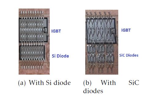Figure 1: An IGBT-diode pair of HybridPACK Drive Module

For the purpose of evaluating the benefits of SiC, a prototype SiC Hybrid module has been produced by replacing the Si diodes of HPD with Generation5 650V SiC Schottky diodes from Infineon [16]. The SiC diodes have a die size of 7.12 mm² and a nominal current rating of 40A. Each of the 50 mm² Si diodes are replaced by a parallel connection of six SiC diodes as seen from figure 1(b), leaving the remaining construction of the module as it is, for a direct evaluation of the SiC diodes vis-a-vis the Si diodes. This module shall be referred to as “HPD-Hyb-SiC” in this paper.

3.1 Inverter  Power  Loss Calculation Model

For a good comparison of the power loss performance of different chip technologies, it is imperative to have an accurate inverter power loss model. This model should offer an uncertainty significantly lower than the performance difference between the technologies compared. For example, it is meaningless to compare two different technologies which differ in loss performance by 20% with a model which suffers from 15% uncertainty, because it is not possible to ascertain if the apparent difference between the technologies is indeed because the technology is better than the other, or if it is merely due to the high uncertainty of the model used. Since this paper would compare Si and SiC technologies which usually differ by 10 to 20 percent, a model with an uncertainty of < ±5% presented in [17, 18] is used and the parameters A₁₁– E₄₃ are determined for both the modules. The parameters for HPD can be found in [17, 18], and those for HPDHyb-SiC in [2].

4 Mission Profile Analysis

The model discussed in the previous section is used to compare the performance of the two modules for 5 different mission profiles, viz., Artemis-Urban, Artemis-Highway, Artemis-Rural, WLTP and NEDC.

For the mission profile investigation, a typical mid size sedan similar to Volkswagen Golf presented in [2] is chosen as the reference vehicle. The results at 8kHz are given in figure 2.

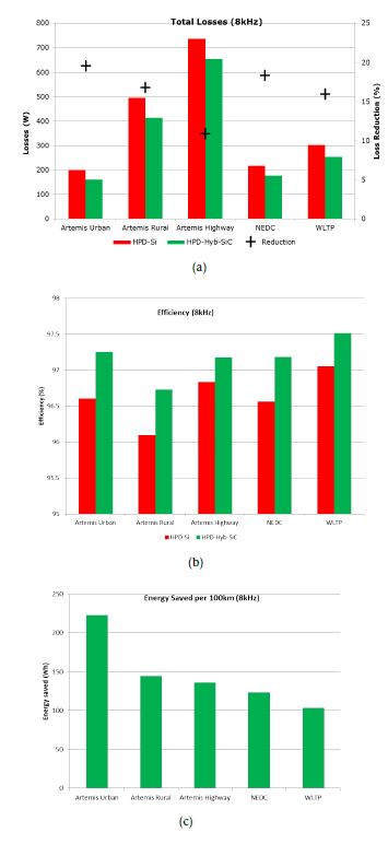Figure 2: Results of Mission Profile Analysis for the modules

As a result of the higher average driving speed, the overall losses are the highest for Artemis Highway driving Cycle. Artemis Urban on the contrary, has the least average losses due to its low average speed. HPD-Hyb-SiC has about 10-20% lower losses compared to HPD-Si. The reduction in the losses is the highest for the Artemis Urban cycle, where the inverter operates in the low current regime. This is because, at low currents the switching losses (which are significantly lesser in the SiC diode compared to the Si diode) dominate over the conduction losses (which are higher in the SiC diodes than the Si diodes). Next, the study is repeated at different switching frequencies, 8-15kHz. The improvement in efficiency of the SiC module over the Si module is summarized in figure 3. Again, the highest benefit of increasing f_sw is for the Artemis Urban drive cycle, which sees more than 1.2% improvement in efficiency at 15kHz compared to about 0.7% at 8kHz. Artemis Rural and Artemis Highway cycles too are not far behind. This is because in all the artemis cycles, the switching losses dominate over the conduction losses, and the scope for improvement with SiC diodes is high. The NEDC and WLTP cycles are mostly dominated by conduction losses, and as a result the benefit of using SiC diodes is not high.

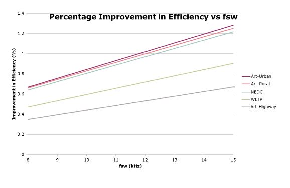Figure 3: Mission Profile analysis at different fsw

5 Experimental Validation of the Behavioral Power Loss Calculation Model

To have a good confidence level in the behavioral power loss calculation model used for mission profile analysis and to verify it experimentally, it is important to measure the inverter power losses at various operating points, preferably with two independent methods. Firstly, power loss measurements are performed at various inverter operating points with the power-analyser based input-output electrical method, which, being relatively easier to perform, is the most commonly used method for such applications. The sources of uncertainty are thoroughly analysed and it will be shown that this method has high uncertainty due to the switched nature of the output voltage waveform. A common solution to this problem is to add a sine output filter. However, the results include also the losses in the filter leading to wrong results, as will be shown in this paper. Thus, it is necessary to resort to the calorimetric method proposed in [3], which is nearly as easy to perform as the electrical method and is particularly suitable for low-lossy conditions.

This method does not require the use of an expensive calorimeter.

6 The Electrical Input-Outputbased Method

6.1 Test Setup

A test platform is built as per the schematic in figure 4. The inverter (described in section 7) is connected to a 3-phase inductive load. The input dc current I_dc and output rms currents I_rms are sensed using high accuracy closed loop current transducers IT 200-S ULTRASTAB [19] and LF 510-S [20] respectively, which are then fed into a state-of-the-art precision Power Analyser WT1800 [21]. WT1800 has a high sampling frequency of 2MHz with 16-bit resolution and a bandwidth of 5MHz. It is also equipped with a digital line filter which can be set for frequencies from 100Hz to 100kHz. The impact of using this line filter on the accuracy will be also discussed later in this paper. The inverter is run in open-loop mode, and the desired output voltage is requested by setting the modulation index accordingly. The power analyser measures the input dc power P_dc and the output ac power P_ac, and the difference is equal to the power loss P_loss, from the basic definition, as per equation 1.

                                     Ploss = Pdc −Pac                                            (1)

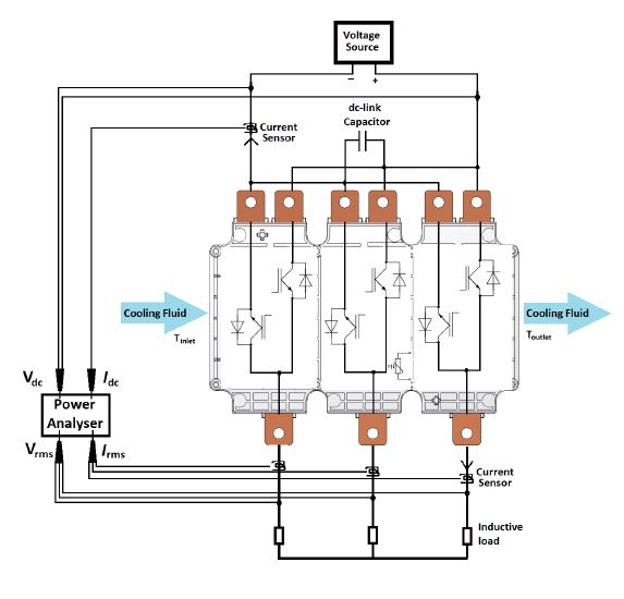Figure 4: Schematic for measurement of power losses with the electrical method

6.2 Sources of Uncertainty

Uncertainties occur in this method, on account of the delays introduced by the probes and unintended phase-shifts between the different measured signals. In this section, the uncertainty involved in this method will be systematically derived. Out of the scope of this work are the errors introduced on account of the Radio Frequency Interference (RFI) and Electro Magnetic Interference (EMI) emanating from the high di/dt and dv/dt prevailing in hard switched power converters.

The uncertainty in the measurement of the power loss ∆P_loss from equation 1 can be derived using the Gaussian law of error propagation.

 

                       ∆Ploss                   ∆Pdc !2 ∆Pac !2

                                   =                      +                                 (2)

                        Ploss                    Pdc                  Pac

Equation 2 gives the uncertainty with a confidence value of about 68%. This will simply be referred to as uncertainty in the rest of this work. The upper bound for the uncertainty ∆P_loss,max can be simply calculated as

                                 ∆Ploss,    max ∆Pdc      ∆Pac

                                              =            +                                (3)

                                Ploss                Pdc           Pac

This will hence be referred to as the maximum uncertainty.

6.2.1       Uncertainty in P_dc

To calculate ∆P_dc, we have to go back to the fundamental equation of dc power, i.e.,

Pdc = Vdc ·Idc   (4)

and the uncertainty can again be calculated by the Gaussian law described above as:

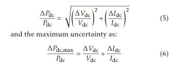
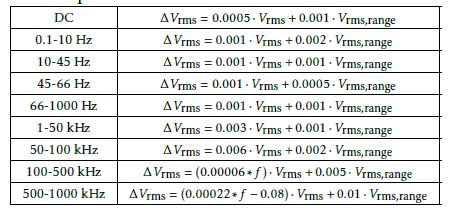
From the reference manual of the power analyser [21], the uncertainties for the dc voltage measurement are given as a function of the set range V_dc,range and the reading itself as follows

∆V_dc = 0.0005·V_dc +0.001·V_dc,range                                           [V ] (7)

Additionally, it must be remembered that there is also a ripple in V_dc consisting mainly of a second harmonic of the fundamental frequency, and small magnitudes of harmonics of the switching frequency. These harmonics also contribute to the uncertainty, as will be covered in section 6.2.2. But, as the magnitude of this ripple is quite small, their contribution to the uncertainty can be neglected.

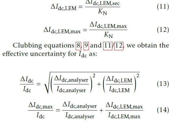
The uncertainties for the measurement of I_dc are similarly given as

∆I_dc,analyser = 0.0005^·I_dc+0.001^·I_dc,range                                  [A] (8)

∆I_dc,analyser, however, is the uncertainty of just the power analyser and since we are using an external LEM current transducer, we also have to take its uncertainty into account. From [19], the uncertainty for the LEM transducer on the secondary side can be given as:

∆Idc,LEM,max,sec = IOE+L^·Ipry,range^·KN   [A] (9) and

           ∆Idc,LEM,sec =            ^I_OE² +(L ^·Ipry,range ^·KN)²                   (10)

where, I_OE = 80 · 10⁻⁶A is the electrical offset current, _L = 3 · 10⁻⁶A is the linearity error,

I_pry,range=200A is range on the primary side and K_N=0.001 is the turns ratio. It is to be noted that, the effects due to self heating in the current transducer are neglected and it is assumed that the transducer is at a constant temperature of 25^◦C. Since we are interested in the primary current for calculating P_dc, the absolute uncertainties get divided by the turns ratio as follows:

 

6.2.2       Uncertainty in P_ac

From the fundamental equation for the ac power for a line-line voltage of V_rms, line current I_rms and a power factor angle φ (in radians),

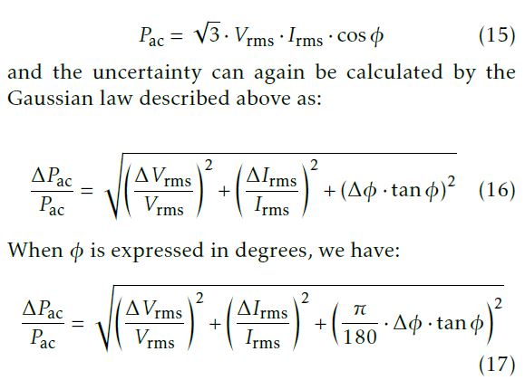
The calculation of uncertainty in the measurement of P_ac is less straightforward than that for P_dc. This is because, the inverter output voltages and currents used for determining P_ac are not pure sinusoids and contain a spectrum of various frequencies, and the uncertainties of the power analyser are differently defined for the spectral components of different frequencies. Moreover, the reference manuals for the power analyser define the uncertainties only for pure sine waves and do not explicitly describe how these spectral components have to be treated. One simplified approach, commonly adopted in literature, is to assume that the output voltage spectrum would be dominated by the fundamental output frequency f_o

and then calculate the uncertainty as if the output voltage were a pure sine wave with f_o. However, as can be expected and as shall be shown later in this paper, such an approach results in a significant discrepancy in the estimation of uncertainty. Therefore, in this work, we propose the following spectrum-based approach.

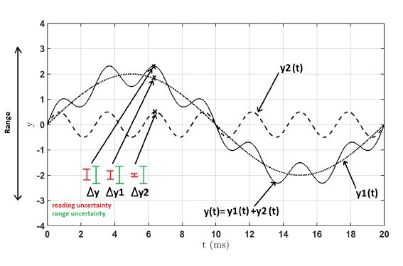
Figure 5: Reading- and range-uncertainties for a summation of signals Spectrum-based Approach to Calculating Uncertainty of Non-sinusoidal Signals

To understand how reading- and range- uncertainties should be calculated for a signal that is a combination of several signals, consider figure 5 which

shows three signals, viz. y₁(t) at 50 Hz, y₂(t) at 350 Hz and y(t)= y₁(t)+y₂(t). Lets assume that all the signals are measured with the same range r. Lets consider the points (t,y₁), (t,y₂) and (t,y) on the three signals respectively. The uncertainties for the three signals are also shown. The reading uncertainties ∆y_1/2,reading can be calculated as follows:

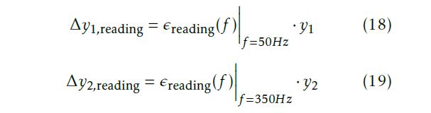
where, _reading(f) is the frequency-dependent reading uncertainty coefficient normally specified in the reference manual. The range uncertainties ∆y_1/2,range can be calculated as follows:

∆y1,range = ∆y2,range = range ^·r (20) where, _range is the uncertainty coefficient for the range, also specified in the reference manual. As the dependency of the range uncertainty on the spectral components is small, it is assumed that _range is independent of f. The reading uncertainty ∆y_reading for the summed signal can be calculated simply by the sum of the reading uncertainties for the two signals as follows: The uncertainties for the three signals are also shown. The range uncertainties ∆y_range can be calculated as follows:

                       ∆yreading = ∆y1,reading +∆y2,reading                     (21)

• A fundamental period of Vac in time domain
• Spectral components
• Reading uncertainty for the spectral components

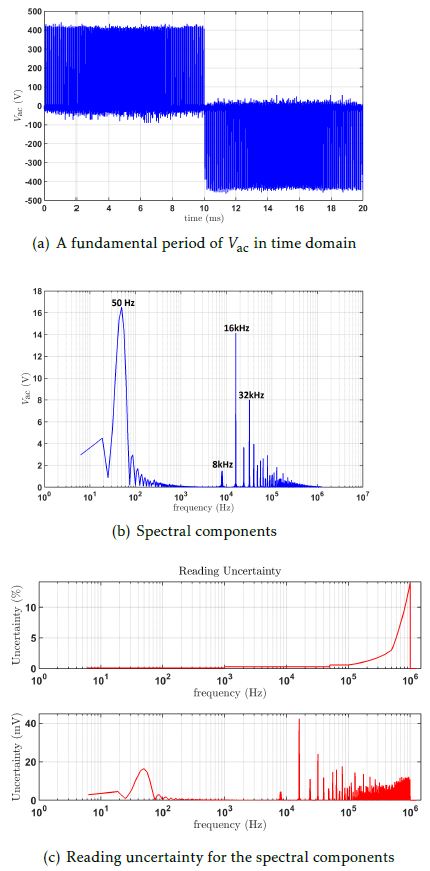Figure 6: Measured output line-line voltage V_ac of a hard-switched inverter

The range uncertainty ∆y_range, however, could be expected to be the same for ∆y as for ∆y_1/2 as we are using the same range. This means that, unlike in the case of the reading uncertainty, the range uncertainty for the sum of two signals is not equal to the sum of

the range uncertainties for the two signals. Therefore, ∆y_range is equal to that calculated by equation 20. Let us now consider a practical example. Figure 6(a) shows one fundamental period of the measured waveform of a typical hard-switched inverter output lineline voltage V_ac. First, the measured voltage waveform is subject to a fourier transformation to decompose it into its spectral components, as shown in figure 6(b). It can be seen that apart from the fundamental frequency 50Hz, there is significant contribution at the switching frequency 8kHz and multiples thereof. The reading uncertainties for the different components are calculated using the respective equations in table 1, as defined by the reference manual. Figure 6(c) shows the calculated reading uncertainty, both absolute and percentage, as a function of the spectral frequency. The original spectrum taking into account the uncertainties is now transformed back into the time domain. The range uncertainty is calculated as described previously and is added to this time-domain signal to yield the required V_ac +∆V_ac.

Table 1: Definition of Uncertainty for different Spectral Components

This spectrum-based approach is also used to calculate the uncertainty for the current I_ac. The measured waveform is shown in figure 7(a). It can be seen that, unlike V_ac, I_ac is nearly sinusoidal which is on account of the inductance of the load. This can also be verified from the frequency spectrum shown in figure 7(b) where it can be seen that most of the energy is concentrated at the fundamental frequency. The contribution of the harmonics of the fundamental and the switching frequency is significantly lesser than in the case of V_ac. The calculated uncertainty as a function of the frequency spectrum is shown in figure 7(c).

The total uncertainties thus calculated for the rms values of V_ac and I_ac are tabulated in table 2^[1]. The approximate approach underestimates the uncertainty in V_ac by a factor of three compared to the spectrum-based approach, due to the abundance of high-frequency content in the waveforms. For I_ac, on the other hand, both approaches result in nearly the same value, owing to the current waveform being nearly sinusoidal. Therefore, it can be summarized that the approximated approach is sufficient for calculating uncertainty in I_ac, but it is necessary to go to the more exact spectrum-based approach for calculating uncertainty in V_ac. Moreover, in applications with a higher switching frequency or a higher operating dc-link voltage V_dc, which is typical for a SiliconCarbide-based application, the uncertainty in V_ac is higher respectively due to a wider distribution in the spectrum and a higher range that has to be chosen. In such applications, a higher deviation can be expected between the approximate and the spectrum-based approach which makes it more meaningful to use the spectrum-based approach.

• A fundamental period of Iac in the time-domain
• Frequency spectrum
• Reading uncertainty for the spectral components

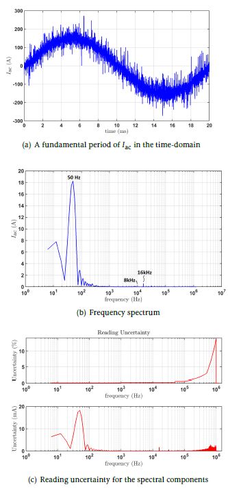Figure 7: Measured line current I_ac

The uncertainty contribution due to the current transducer ∆I_rms,LEM can be calculated as follows:

∆Irms,LEM = 0.005^·Irms,nom                (22)

where, the nominal current I_rms,nom=500A for the device used. The uncertainty ∆I_rms can be now written as

Table 2: Calculated measurement uncertainty for V_rms and I_rms

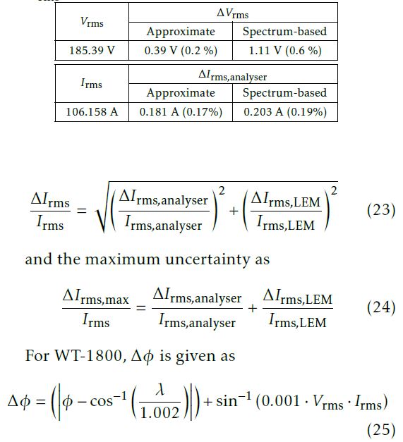
where λ is the power factor. Lastly, it has to be remembered that the uncertainty of the power analyser depreciates over the passage of time from its recent calibration. For WT-1800, the uncertainty at one year is 1.5 times that at 6 months.

A Common Measurement Mistake while applying Line Filters in Power Analysers Most state-of-the-art power analysers come equipped with digital line filters which can be used to attenuate spectral components in the measured signals with a frequency higher than a certain cut-off frequency (generally programmable individually for each input channels). These filters are meant to be used on measurement signals where there is high frequency noise due to the limitation of the measuring equipment. Let us suppose that such a filter is used on the I_ac signal with a cut-off fequency of, say, 1kHz. The high frequency components in I_ac are predominantly due to measurement noise as can be seen from figure 7(b) and table 2, and using such a filter would help in attenuating this noise, thereby making the measurements more meaningful. However, suppose we use the same filter, either intentionally or accidentally, on V_ac which inherently has a high-frequency content (see figure 6(b) and table 2), other than measurement noise. In such a case, the filter would attenuate not only the noise, but also these high frequency components. This would, in turn, result in a lower-thanreal measured value for P_ac and therefore, a higher P_loss. Therefore, the line filter should be used only on signals which do not inherently have high frequency components, like V_dc, I_dc and I_ac, but not on signals like V_ac which have a high frequency content. This is a common mistake while performing measurements incorporating such line filters, and will be demonstrated in the next section 6.3.

6.3 Measurement Results

Figures 8-12 show the power losses measured with the electrical method for different application conditions. The uncertainties calculated for each of the measurements, using the spectrum-based approach described in the previous section, are shown as bars around the measurement points. Also shown are the simulated results based on the behavioral model discussed previously, and the relative deviation of the measured values from the simulation.

Figure 8(a) and 9(a) show P_loss measured for different output rms currents, I_rms, at V_dc=100V and 300V respectively. Across the entire range of the measured current, it can be seen that the simulations are within the tolerance of this state-of-the-art electrical input-output measurement approach, thereby validating the behavioral power loss calculation model.

In figures 10(a) and 11(a), the results are shown for different values of the gate resistances R_g,on and switching frequencies f_sw. It can again be seen that the simulations are within the tolerance of this stateof-the-art input-output measurement approach.

• Ploss
• Relative Deviation (%)

Figure 8: Comparison of the electrical method with simulations: P_loss vs. I_rms at V_dc=100V

• Ploss
• Relative Deviation (%)

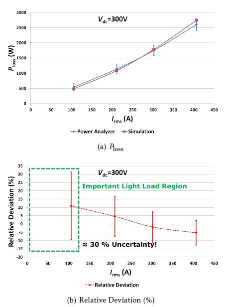Figure 9: Comparison of the electrical method with simulations: P_loss vs. I_rms at V_dc=300V

• Ploss
• Relative Deviation (%)

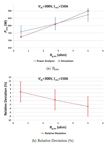Figure 10: Comparison of the electrical method with

simulations: P_loss vs. R_g,_on

Lastly, figure 12 shows the measurements performed with the line filter (cut-off frequency=1kHz) enabled for the output ac voltage V_ac, and compares them with the measurements without the filter. As explained in section 6.2.3, it can be seen that the losses measured are higher without the line filter because the measured P_ac is lower-than-real. This shows that enabling the line filter on V_ac can lead to wrong measurements. Overall, it must be observed that the electrical input-output based method has nearly 30% uncertainty in the light-load condition, making this method unsuitable for the main inverter application, especially when comparing different chip generations.

• Ploss
• Relative Deviation (%)

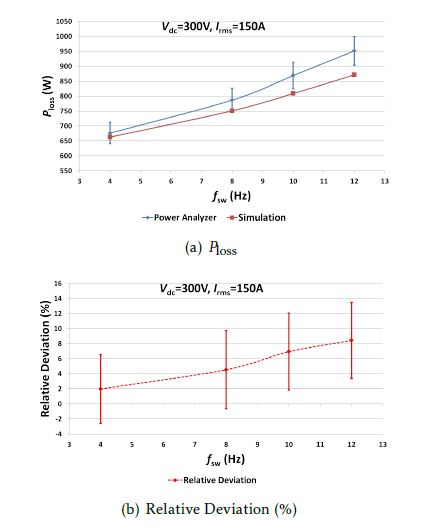Figure 11: Comparison of the electrical method with simulations: P_loss vs. f_sw

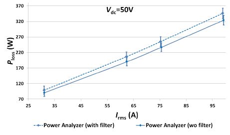
Figure 12: Comparison of the electrical method with simulations: Effect of Line Filter

7 Calorimetric Measurement of Power Losses

A more accurate approach, compared to the electrical method, is to measure power losses with a calorimeter [22]. For applications such as the automotive main inverter which operate at less than a quarter of the inverter nominal current more than 90% of the time[17], the light-load low-lossy condition is of interest. With traditional calorimetric methods, however, a sufficient rise in the fluid temperature is hard to obtain at these conditions. To overcome this problem, without compromising on the accuracy, the inverter is subjected to a calorimetric method particularly suitable for low-lossy conditions. This method does not require the use of an expensive calorimeter and is presented in detail in [3]. A requirement for the test is that all the energy losses in the module must ideally go into heating up the baseplate, with no convection. Therefore, the module baseplate is thermally insulated with a layer of polystyrene as can be seen in figure 13. EVAL-6ED100HPDRIVE-AS, a 6-channel gate-driver board based on the EiceDriver 1EDI2001AS from Infineon, is connected on the top of the module. The gate-driver board is controlled by a micro-controller logic board connected on top of it. The logic board is connected to a computer through a CAN bus, and the parameters such as f_sw, m, f_out can also be controlled by software, in open loop or closed loop modes. Moreover, it is also possible to read the temperatures sensed by the NTCs and log them. The complete inverter system is shown in figure 14. This method comprises the following two stages.

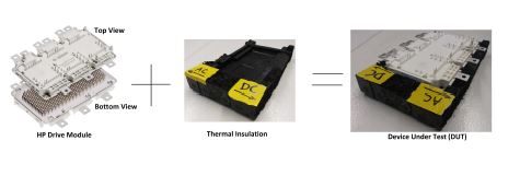Figure 13: The DUT with the Thermal Package for the Calorimetric Test Bench

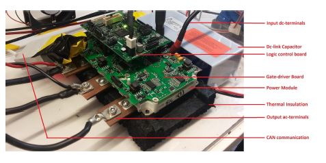Figure 14: The Complete Inverter System in the Calorimetric Test Bench with the Thermally Isolated Baseplate

7.1 Calibration Stage

In this stage, the inverter system is connected to a dc source (with opposite polarity) with voltage sense pins capable of serving as a constant power source. The output ac terminals are disconnected as shown in the schematic in figure 15(a). A known amount of constant power P_cal is injected into the module through the diodes. As there is no output power, all the injected power is dissipated in the module as heat, which is trapped in the heatsink on account of the thermal insulation, as seen in figure 15(b). As the temperature of the diode increases, its voltage drop changes and the dc source must be capable of suitably adjusting the current to maintain the power constant. Due to the thermal insulation, and the absence of convection, almost all the heat is trapped in the capacitance of the baseplate, and goes on to increase its temperature exponentially as shown in figure 16(a).

• Schematic Diagram
• Thermal Stack

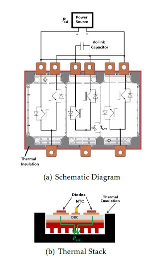Figure 15: Calibration Setup

There is a small amount of heat that is radiated into the ambient, or leaves the modules through any surface other than the heatsink. However, this effect will be cancelled out and have no impact on the accuracy of this method if the test setup during the calibration and measurement stages is identical. The temperature sensed by the NTCs is recorded until it rises from T₁ = 50°C to T₂ = 90°C^[2], after which the dc source is switched off and the system is let to cool down to the ambient temperature. In order to filter out measurement noise, an exponential curve is fitted to the measurement. From this fitted curve, the time taken for the temperature to reach T₁ from T₂ is taken as the rise time t_r. The temperature slew rate s_r is calculated as

sr = T2 −T1         (26) tr

This experiment is repeated at different values of injected power and P_cal is plotted against s_r as shown

in figure 16(b) for both the modules and first order curves are now fitted to the two curves respectively, and the equations of the fitted curves are given below:

P_loss = 249.68·s_r+48.655                            [HPD Module] (27)

P_loss = 258.15·s_r +45.905                    [HPD-Hyb-SiC Module] (28)

As seen in figure 16(b), the calibration curves for the two modules match very closely, owing to the similar construction of the module. This is in line with the objective of this work to have minimum discrepancies arising out of differences in the packaging, for a fair comparison of Si and SiC. The slight difference seen between the curves can be attributed to the difference in the NTCs and the temperature measurement tolerances, which are cancelled out due to this method.

• NTC temperature at Pcal =100W
• Calibration Curve

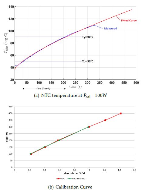Figure 16: Calibration

7.2 Measurement Stage

In this stage, the inverter is connected to a dc voltagesource (with normal polarity). Care must be taken to see that the setup, particularly the thermal insulation, is not disturbed between this stage and the calibration stage. The output ac terminals are connected to a three-phase star-connected passive load as shown in figure 17 and the inverter is run in open-loop mode. A suitable rms current I_rms is established in the load, by adjusting m appropriately. As with the calibration stage, s_r is determined.

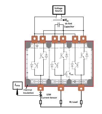Figure 17: Measurement Stage

• Ploss
• Relative Deviation (%)

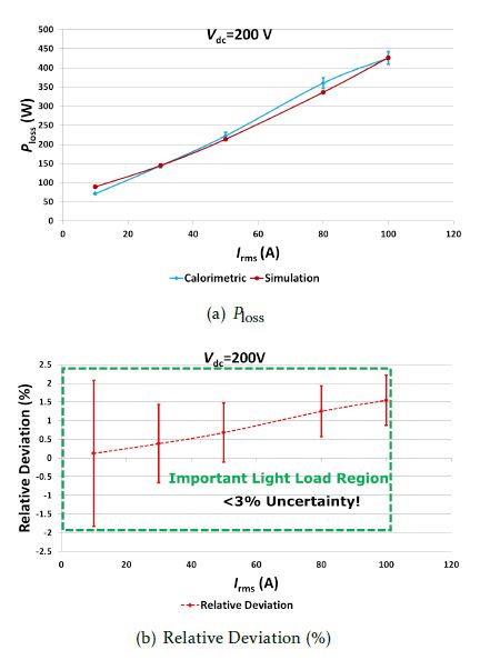Figure 18: Comparison of the calorimetric method with simulations: P_loss vs. I_rms at V_dc = 200V

Now, the inverter losses can be obtained by substituting the measured s_r in equation 27 and 28 obtained from the calibration stage. The inverter power losses for different I_rms at two different working voltages 200V and 400V measured for HPD with the proposed calorimetric method are shown in figures 18(a) and 19(a). These are compared against simulations at the respective points. Also shown are the calculated uncertainties (this topic is described in [3]) for each of the points as bars around the measurement points. The relative deviation between the measurements and the simulations, expressed as percentage, is shown in figures 18(b) and 19(b). Across the entire range of measurement, it can be seen that the simulations are within the tolerance of the calorimetric approach, again validating the behavioral simulation model. Furthermore, in each of these cases, it can be seen that the uncertainty is well below 5%, especially at partial-load which makes the calorimetric method suitable for automotive main inverter applications, particularly for comparing chip technologies whose total power losses may differ in the range of 1020%.

• Ploss
• Relative Deviation (%)

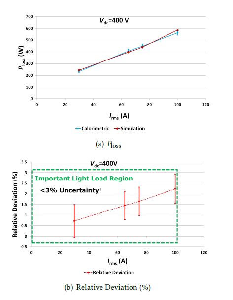Figure 19: Comparison of the calorimetric method with simulations: P_loss vs. I_rms at V_dc = 400V

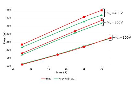Figure 20: Measured Inverter Losses vs I_rms at various V_dc for HPD and HPD-Hyb-SiC

7.2.1 Comparison of Measured Inverter Losses for HPD versus HPD-Hyb-SiC

The tests are repeated for different operating points of V_dc, I_rms and f_sw for both the modules. Figure 20 shows a summary of the measured losses as a function of I_rms at different dc-link voltages. It can be seen that at V_dc=100V, the SiC module has almost the same losses as the Si module, offering no benefit. This is because at low V_dc, the switching losses do not contribute much to the total losses, and the conduction losses are dominant. As the conduction losses are higher in the SiC diodes as can be seen from the static curves presented in [2], HPD offers better overall performance than HPD-Hyb-SiC. At V_dc=300V, the benefits of SiC become prominent. At V_dc=300V, I_rms=75 A, there is about 5% reduction in the total losses. This gap widens as we increase V_dc as the switching losses become more dominant, and at V_dc=400V, 75A, we can see a reduction of around 7%.

8 Conclusions

In this paper, the benefits of replacing the Si diodes of a commercial automotive IGBT module with SiC diodes have been investigated for the main inverter application, maintaining the operating conditions, package and the rest of the system the same, to ensure a fair comparison of the devices without any external influence. A behavioral power loss model, suitable for mission profile analysis, is used to compare the performance of the two modules over several mission profiles. The highest benefit of using SiC diodes is seen for the Artemis Urban drive cycle, where the SiC diodes help reduce the overall losses by 20% at f_sw=8kHz. This translates to a saving of around 200Wh of battery energy per 100km. The behavioral model is experimentally verified by comparing it against two independent measurement methods, namely, electrical input output method and a calorimetric method. In each case, the simulation results are found to be within the tolerance of the measurements, thereby validating the simulation model used. At V_dc =400V, I_rms =75A, the inverter losses were found to be reduced by over 5% with the SiC module, due to the absence of reverse recovery in the unipolar SiC schottky diodes. This reduction is even better at higher dc-link voltages, due to the switching losses becoming more prominent.

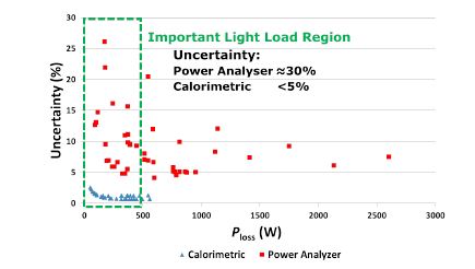Figure 21: Scatter Plot of the uncertainties (%) at various measurement points for the two methods vs P_loss

Further, as summarized in figure 21, it can be concluded that the commonly used power analyser based electrical method has an uncertainty of nearly 30% in the light load condition, mainly due to delays and phase-shifts in the probes. It is to be noted that automotive traction inverters operate most of the time in the light-load condition, which means that the electrical method is not suitable for such applications. The developed calorimetric method outperforms the standard electrical input-output based method and achieves, especially in the important light-load region, a measurement uncertainty of lower than 5%. Furthermore, as the expensive calorimeter is not required for this method, it is nearly as easy to perform as the power-analyser based electrical method. This makes it ideal for comparing device technologies such as Si versus SiC in automotive main inverter applications.

9 Future Work

This work considered the advantages of replacing only the diodes with SiC. However, for higher benefits, it is desirable to replace the IGBTs with SiC MOSFETs, and it would be interesting to investigate the benefits they bring in terms of higher efficiency for different mission profiles. This will considered in a future publication.

• As with Idc, we are using an external LEM current transducer for measurement and therefore, we must separately calculate the uncertainties ∆Irms,analyser and Irms,LEM for the power analyser and the LEM transducer [20] respectively.
• The choice of T1 = 50°C and T2 = 90°C is based on the observation that between these temperatures, the exponential curve is nearly linear. However, a different set of values may be chosen, provided that the temperature rise curve is nearly linear in this interval. But it must be ensured that the temperature limits chosen during calibration and measurement stages are the same.

1. Ajay Poonjal Pai, Tomas Reiter, and Martin Maerz. Mission profile analysis and calorimetric loss measurement of a sic hybrid module for main inverter application of electric vehicles. In Integrated Power Packaging (IWIPP), 2017 IEEE International Workshop On, pages 1–5. IEEE, 2017.
2. Ajay Poonjal Pai, Tomas Reiter, and Martin Maerz. Characterization and mission profile analysis of a SiC hybrid module for main inverter application of electric vehicles. In EEHE 2017 Bamberg; Proceedings of. Haus Der Technik, 2017.
3. Ajay Poonjal Pai, Tomas Reiter, Oleg Vodyakho, Inpil Yoo, and Martin Maerz. A calorimetric method for measuring power losses in power semiconductor modules. In EPE 2017Warsaw; Proceedings of. ECCE Europe, 2017.
4. Kimimori Hamada. Great potential of SiC devices for environmentally friendly vehicles. In APE Automotive Power Electronics. IEEE, 2015.
5. Ming Su, Chingchi Chen, Shrivatsal Sharma, and Jun Kikuchi. Performance and cost considerations for SiC–based HEV traction inverter systems. In Wide Bandgap Power Devices and Applications (WiPDA), 2015 IEEE 3rd Workshop on, pages 347–350. IEEE, 2015.
6. Benjamin Wrzecionko, Dominik Bortis, and Johann W Kolar. A 120 C ambient temperature forced air–cooled normally–off SiC JFET automotive inverter system. IEEE Transactions on Power Electronics, 29(5):2345–2358, 2014.
7. SK Singh, F Gu´edon, PJ Garsed, and RA McMahon. Halfbridge SiC inverter for hybrid electric vehicles: Design, development and testing at higher operating temperature. In Power Electronics, Machines and Drives (PEMD 2012), 6th IET International Conference on, pages 1–6. IET, 2012.
8. Fei Shang, Alejandro Pozo Arribas, and Mahesh Krishnamurthy. A comprehensive evaluation of SiC devices in traction applications. In Transportation Electrification Conference and Expo (ITEC), 2014 IEEE, pages 1–5. IEEE, 2014.
9. Justin K Reed, James McFarland, Jagadeesh Tangudu, Emmanuel Vinot, Rochdi Trigui, Giri Venkataramanan, Shiv Gupta, and Thomas Jahns. Modeling power semiconductor losses in HEV powertrains using Si and SiC devices. In 2010 IEEE Vehicle Power and Propulsion Conference, pages 1–6. IEEE, 2010.
10. Hui Zhang, Leon M Tolbert, and Burak Ozpineci. Impact of SiC devices on hybrid electric and plug-in hybrid electric vehicles. IEEE transactions on industry applications, 47(2):912–921, 2011.
11. Burak Ozpineci, Madhu Sudhan Chinthavali, Leon M Tolbert, Avinash S Kashyap, and H Alan Mantooth. A 55-kW threephase inverter with Si IGBTs and SiC schottky diodes. IEEE Transactions on industry applications, 45(1):278–285, 2009.
12. M Chinthavali, Leon M Tolbert, Hui Zhang, Jung H Han, F Barlow, and Burak Ozpineci. High power SiC modules for HEVs and PHEVs. In Power Electronics Conference (IPEC), 2010 International, pages 1842–1848. IEEE, 2010.
13. Timothy Junghee Han, Jim Nagashima, Sung Joon Kim, Srikanth Kulkarni, and Fred Barlow. Implementation of a fully integrated 50 kW inverter using a SiC JFET based six–pack power module. In 2011 IEEE Energy Conversion Congress and Exposition, pages 3144–3150. IEEE, 2011.
14. Florian Hilpert, Klas Brinkfeldt, and Stefan Arenz. Modular integration of a 1200 V SiC inverter in a commercial vehicle wheel–hub drivetrain. In Electric Drives Production Conference (EDPC), 2014 4th International, pages 1–8. IEEE, 2014.
15. Product brief HybridPACK drive. Infineon AG, 2014.
16. Datasheet 5th generation thinQ 650V SiC schottky diode IDW40G65C5, author=, journal=Infineon AG, year=2013.
17. Ajay Poonjal Pai, Tomas Reiter, and Martin Maerz. A new behavioral model for accurate loss calculations in power semiconductors. In PCIM Europe 2016; Proceedings of. VDE, 2016.
18. Ajay Poonjal Pai, Tomas Reiter, and Martin Maerz. An improved behavioral model for loss calculations in automotive inverters. In EEHE 2016 Wiesloch; Proceedings of, pages 412–427. Haus Der Technik, 2016.
19. Lem current transducer IT 200-S ULTRASTAB, author=, journal= LEM, year=2014.
20. Lem current transducer LF 510-S, author=, journal=LEM, year=2015.
21. Yokogawa WT1800 getting started guide, author=, journal= Yokogawa, year=2015.
22. Xiao, G. Chen, and W. G. H. Odendaal. Overview of power loss measurement techniques in power electronics systems. IEEE Transactions on Industry Applications, 43(3):657–664, May 2007.

(Click to view)

(Click to view)