1. Introduction

Several tuning techniques coexist nowadays for industrial controllers. Ranging from classical frequency domain methods for single loops to state-space controller synthesis, there is an ever-increasing number of design options. Nevertheless, some of these techniques yield no practical value in industry. This is due to inconvenient implementation, computational complexity and the prior background knowledge required in some cases. Usually, these issues are dealt concurrently with a fast-paced industrial environment, where keeping production rates is mandatory. In addition, most industries lack testing facilities or even a reliable process simulator to study in detail different control schemes. Which is more, knowledge in advanced control theory is rather rare among plant engineers.

This work is an overview of different tuning techniques which may be of industrial interest. Based on a real plant, it aims to provide insight into the possible issues of simpler tuning methods, and the effort needed to overcome these issues with more complex techniques. In this regard, four methods were selected with an increasing degree of complexity. To start with SLT, which is a basic Single Input Single Output (SISO) approach. In the second place, BLT method improves closed-loop stability, as proposed by Luyben [1]. Besides, SRD tuning takes into account loop interactions to some degree. Finally, S-H_∞ method belongs to the well known H_∞ theory, which is a rigorous scheme for controller synthesis [2], [3].

It is straightforward that selected methods are quite dissimilar. This was purposely set, as the goal is to find the method with a right trade-off between industrial needs and tuning effort. For this purpose, it is meaningful to highlight advantages and drawbacks of each procedure. Although the analysis is subject to a particular plant, it is still possible to arrive some general conclusions.

Due to the hegemony of Proportional-Integral (PI) control in the industry [4], all of the controllers in this work belong to this type. Furthermore, using the same control structure provides a common framework for tuning method comparison.

This paper is organized as follows. Section 2 describes the problem under study. Section 3 examines relevant features of the steam generator model, and how they may impact on control objectives. A review of selected tuning methods is presented in Section 4. Afterwards, Section 5 provides a discussion over performance results for each tuning procedure. Finally, conclusions are presented in Section 6.

2. System Under Study

A thermal power station must be able to alter its output to meet a varying load demand. At the core of this process lies a Steam Generator (SG). This device regulates steam feed to the turbine, which in turn is responsible for electricity generation. A good tracking of reference command signals is essential for a proper operation. Equally important are plant stability and disturbance rejection. Each of these objectives impact on production costs and operational safety.

The steam generator model under study was originally reported by Tan, Marquez and Chen [5], and later studied by Adam and Valsecchi [6]. This SG is part of cogeneration systems of Syncrude Canada Ltd. integrated energy facility located in Mildred Lake plant site, Canada. Although the model is a simplification, it retains the typical attributes of an SG. Some of these are the multivariable nature and the presence of integrators in the MIMO transfer function.

The model is represented by a 3×3 transfer function matrix. The inputs variables are listed below

u₁: Feed water flow rate (kg/s) u₂: Fuel flow rate (kg/s) u₃: Attemperator spray flow rate (kg/s)

While the output variables are y₁: Drum level (m) y₂: Drum pressure (MPa) y₃: Steam temperature (^◦C)

Figure 1 shows a simplified diagram where these variables are indicated.

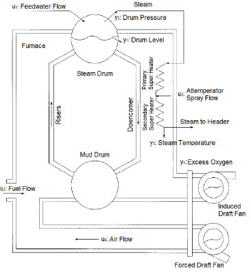Figure 1: Steam generator diagram

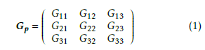
Transfer function matrix is shown in (1), where every G_ij represents the transfer function from input variable i to output variable j.

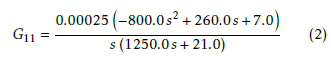
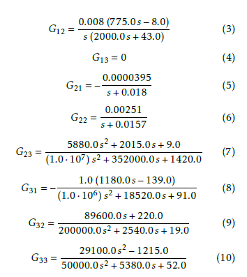
Explicitly, the transfer functions are given by the following expressions

2.1. Operating Point

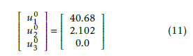
The operative conditions that assure a proper functioning of the boiler system in steady state are the following

Whereas the corresponding output variables are

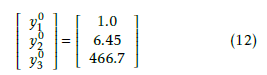Notice that units for each variable were previously defined. Interestingly, attemperator spray flow rate is normally zero. The reason is that the attemperator is used only for precise regulation of steam temperature in transient states. Any other usage of this flow rate leads to higher operative costs.

2.2. Constraints

Plant control system is subject to the following limit constraints

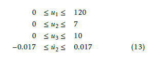It is worth noting that u₁⁰ in (11) is relatively small compared with the magnitude limit in (13), so this limit does not impose a hard constraint for design. However, this is not the case for u˙₂, as limits for fuel flow rate have a remarkable impact on the system performance.

3. Preliminary Analysis

The following paragraphs outline preliminary results of the open loop SG model. A prior characterization of the plant is advisable in order to achieve a better control design. This is due to the fact that it helps to be aware of possible issues beforehand.

3.1. Open loop stability

Open loop stability constitutes an relevant feature in terms of preliminary control design. In particular, an unstable plant leads to special considerations, both for control tuning and plant operation. In this case, the SG model presents integrator modes in matrix elements G₁₁ and G₁₂. Consequently, these elements are not Bounded Input Bounded Output (BIBO) stable for the open loop configuration [7]. Moreover, G_p is a singular matrix in steady state.

3.2. Minimum Phase

It was found that the system is non minimum phase through evaluation of Smith-McMillan transmission zeros [8], as some of the zeros revealed positive real part. Therefore, an inverse response to certain input may occur. The presence of this phenomena can strongly affect control system performance.

3.3. Interactions

Some common problems of multivariable control arise from interactions between inputs and outputs. A proper identification of these enables to select the most effective input-output channels for control purposes. In this regard, a well-known analysis is the so-called Relative Gain Array (RGA), originally proposed by Bristol [9]. However, the presence of integral modes prevents from applying this method, as steady-state gains K_ij are not defined. An alternative algorithm for computing RGA was proposed by Hu, Cai and Xiao [10]. This generalization of the original method is capable of handling both integrator and differentiator modes. According to the algorithm proposed by Hu, Cai and Xiao, RGA is equal to

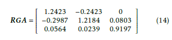The RGA matrix is only meaningful for steady-state interactions. This result confirms that input-output pairing suggested by Tan and Marquez [5] is suitable. Therefore, controlling output i through input i give the best results for every i = 1,2,3. On the other hand, RGA suggests that no severe interactions are present. This is essential in order to reach a good control system performance.

3.4. Directional Sensitivity

A significant difference between the minimum and the maximum singular values was found for the entire frequency band of interest. Consequently, the system is highly sensitive to the direction of input vector. This difference can be verified in Figures 2 and 3, where maximum and minimum singular values are respectively shown. For this reason, control performance may decline according to both magnitude and direction of the input vector [11]. In principle, this justifies the use of MIMO (Multi-Input Multi-Output) techniques for achieving a better control performance.

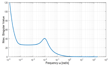Figure 2: Maximum singular value

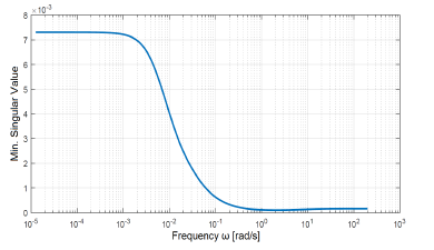Figure 3: Minimum singular value

3.5. Condition Number

As a consequence of this directional sensitivity, condition number is somewhat high, specially in the low frequency range. Consequently, it is expected a certain degree of ill-conditioning [12]. This is shown in Figure 4, where condition number remains moderate-high between frequencies of 1×10⁻⁴ and 1×10¹ rad/s. Also, there is a rapid increase below 1×10⁻⁴ rad/s. In particular, a steady state condition number cannot be even calculated, due to the presence of integral modes in the system.

Special caution must be taken whenever illconditioning is identified, as it is associated with numerical error propagation. Under these circumstances, both analysis and synthesis may result misleading. In order to avoid this issue, calculation algorithms were developed by taking into account numerical error propagation. Additionally, results were validated by crosschecking outputs from different algorithms, whenever this was possible.

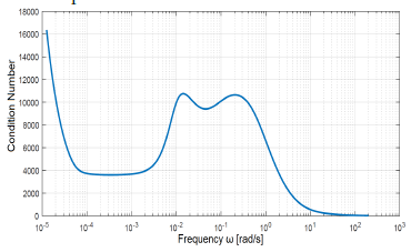Figure 4: Condition number as a function of frequency

Despite the fact that condition number is somewhat high, the RGA reveals that the system has not strong interactions. These findings are actually not in contradiction. On the one hand, condition number is only a measure of the worst possible effect of input direction over the gain of the system. On the other hand, the elements of RGA are relative gains. As such, they are independent of input-output scaling. Additionally, RGA gives information of steady-state plant, whereas condition number is analyzed as a function of frequency.

4. MIMO Tuning Methods

The following paragraphs outline the theoretical frameworks of selected tuning methods.

4.1. Single loop approach

Independent loop tuning is probably the most basic approach, as it only employs classical SISO control design procedures. According to SLT, an input variable is chosen in order to control a particular output variable. Then a control loop is closed for the input-output pair selected. It is worth pointing out that only an element G_ij of transfer function matrix is involved in the loop. Following this, the controller is tuned until reaching the expected response. Finally, the process is repeated for the remainder input-output channels.

This simple procedure allows a tuning optimization for each SISO control loop. However, for the MIMO system, there is no guarantee of good performance, let alone optimality. This is especially true when inputoutput couplings are significant. Nonetheless, this approach became attractive for plant engineers, mainly due to its great simplicity. In turn, this popularity set this approach as a good starting point for comparison between different tuning methods.

4.2. Biggest Log Tuning Method

BLT method was originally proposed by Luyben [1] and remained as a suitable tuning technique in an industrial environment. One of the main reasons for this permanence is that BLT method relies on the logic of single-loop approach, so it holds the advantages of simplicity while considering multivariable coupling to some extent. In fact, a SLT method must be performed as a first step, using specifically the Ziegler-Nichols closed loop method for each control loop. Then the set of PI controllers is detuned in order to satisfy a stability criterion. This semi-empirical criterion is based on the logarithm of the complementary sensitivity function, as stated in [1]. In addition to the advantages of singleloop tuning, BLT procedure returns a robust design, with enough stability margins for the majority of cases. However, as it occurs with the SLT approach, stability is not theoretically guaranteed, because the method depends on a semi-empirical criterion. Another disadvantage is that design may result to be overly conservative. This is a consequence of computing the multivariable coupling in an indirect way, that is to say, through the complementary sensitivity function. Moreover, the dynamic response of control system may result too slow, due to an excess of robustness. Finally, Adam and Valsecchi [6] showed that BLT method might result troublesome when in presence of integral modes in the transfer function matrix. This fact was also regarded by the authors of BLT method.

It must be mentioned that Ziegler-Nichols closed loop method cannot be applied to the SG model selected. This is due to the fact that the resulting characteristic equation leads to a negative ultimate gain and an imaginary ultimate frequency. This means that the system will not exhibit oscillations for any value of proportional gain. For these reasons, the initial values of PI controllers were obtained from the results of the implemented SLT method.

4.3.  Sequential return-difference

Sequential return-difference was first proposed by Mayne [13] and constitutes a variation of the general framework of sequential tuning method.

This variation represents a first step in acknowledging loop interactions. In this approach, a first inputoutput pair is selected in order to close the associated loop. Then a second input-output channel is chosen for closing the following loop while embedding the former control loop. This procedure continues until every channel is reached.

In sequential tuning, loop interactions are only taken into account partially, as it depends on the order of selected channels. In other words, the last closed loop is adjusted considering its effects on the remainder loops; but this is not the case for rest of the loops. Particularly, the first closed loop does not contain any information about the rest of the plant. Notwithstanding this limitation, this approach is potentially very convenient in industrial practice. In this regard, sequential return-difference provides an improvement, as it introduces a cross-coupling stage of compensation. This stage may consist of either a constant-gain matrix or a sequence of elementary operations, and its purpose is to distribute the ”difficulty of control” among the loops [8].

It is worthwhile noting that, as with the previous methods, sequential return-difference offers no guarantee of stability, nor even a good performance is assured.

4.4.  Structured H_∞ method

Theory of H_∞-control started with the work of Zames [14]. Since then, several methods were derived to synthesize controllers that achieve stabilization with guaranteed performance. While some of these techniques were formulated in state-space representation, others belong to the frequency domain. In any case, they all feature an optimization problem, by minimizing an H_∞-type norm of a certain cost function.

Nonetheless, H_∞ methods usually yield non structured, high order controllers, even when some of these methods consider structured uncertainty, like µ-synthesis. Non structured controllers are difficult to implement in practice. Also, controller equation generally lacks integral action [12]. To avoid these drawbacks, in this work we adopted the approach given by Apkarian and Noll [2]. This is the first formulation suited to obtain structured controllers, such as PID, which have a straight industrial instrumentation. Hence this strategy is known as Structured-H_∞ Synthesis. At the core of this method, minimization of a non smooth, non convex and discontinuous functional must be performed. This optimization is an NP-hard problem, so it requires both computational power and attention to convergence issues, being these the main disadvantages. Among the benefits, PID controllers are optimized, in contrast with classical theory, were controllers are simply tuned. Additionally, the resulting controller stabilizes internally the control system [12]. Finally, this method admits constraints in the design problem, an important feature in practical applications.

5. Results

5.1. Controller Parameters

Table 1 reports controller parameters obtained with each of the methods previously introduced. Notice that

SLT gains are generally higher. This suggests a faster dynamics, but also a less robust design. However, robustness may be highly desirable in the presence of loop interactions and process variability, just to name a few potential issues.

On the other hand, BLT method presents lower gains and higher integral time constants than SLT procedure. This is expected, as BLT aims to improve robustness by detuning SLT parameters.

A remarkable feature of SRD values is its parameter variability. Particularly, integral times differ up to five orders of magnitude. This might be possibly due to the cross-coupling stage of compensation, which was mentioned above.

Table 1: PI controller parameters

SLT	BLT	SRD	S-H∞
K1            1.74·103	5.46·102	2.86·102	1.16·102
K2            6.52·100	2.03·100	8.10·10−2	2.34·100
K3 -6.01·10−2	-1.88·10−2	-4.19·10−2	-1.07·10−1
T1            6.01·101	1.92·102	1.78·106	2.61·102
T2            2.12·101	6.79·101	8.77·104	4.54·101
T3            9.37·101	2.99·102	4.43·101	1.66·102

Finally, it is worth noting that all parameters of the same type and controller share the same sign. This reflects a qualitative similarity between such diverse methods.

5.2. Integral Performance

Performance assessment is essential in control systems.

A first step in this field is achieved by using Integral Performance Indexes (IPI). Among these widely used measures, Integral Square Error (ISE) and Integral Time Absolute Error (ITAE) were selected. Both approaches have a long tradition in the literature, and they provide complementary information to some extent. While ISE method penalizes error magnitude, ITAE give a trade off between error and settling time. Table 2 shows a comparison for the resulting control systems, taking only into account diagonal elements, that is

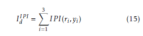where IP I can be either ISE or ITAE. The sum I_d^IPI only takes into account loops with paired variables, that is, with input r_i and output y_i. Both variations of I_d^IPI constitute global measures of tracking quality for the MIMO control system.

Table 2: IPI for diagonal elements – Tracking problem.

Method	ISE %	ITAE %
SLT	20	1
BLT	100(1)	100(2)
SRD	31	34
S-H∞	46	15

⁽¹⁾100% ISE corresponds to 3.98×10²

⁽²⁾100% ITAE corresponds to 5.74×10⁵

Table 2 presents ISE and ITAE percentage values, relative to the highest value for every IPI. As it is shown, SLT exhibits a better IPI behavior, even by orders of magnitude. This is in fact not unexpected, as tracking performance is the main criteria for tuning controllers with SLT. Regarding ISE, SRD follows in performance, while the second place is S-H_∞ with respect to ITAE index. Finally, BLT scores the worst performance in both cases.

To conclude, SLT exhibits the best averaged tracking, either with respect to quadratic deviations (ISE) or weighed along time (ITAE).

By the other hand, integral indexes can be summed for every input-output pair in control system, and the resulting quantity

reveals information about disturbance rejection, as diagonal integrals are negligible with respect to non diagonal ones. Table 3 presents these data as percentages, relative to the highest value for every IPI.

Table 3: IPI for whole system – Disturbance rejection

Method	ISE %	ITAE %
SLT	11	2
BLT	100(1)	100(2)
SRD	20	21
S-H∞	3	5

⁽¹⁾100% ISE corresponds to 1.83×10⁷

⁽²⁾100% ITAE corresponds to 2.58×10⁸

Following Table 3, S-H_∞ method shows the best disturbance rejection under ISE criteria, while SLT holds the first place with respect to ITAE index. Once again, BLT method shows the worst performance.

5.3. Dynamic Response

Even when integral performance offers valuable information, it is still useful to examine dynamic behavior of each system. Starting with the tracking problem, Figure 5 exhibits drum level response against a step of 10% increase in level setpoint. Similarly, Figure 6 shows drum pressure response after a step of 5% increase in pressure setpoint. Finally, Figure 7 presents steam temperature following a step of 10% increase in temperature setpoint.

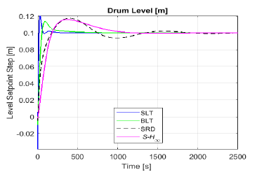Figure 5: Step response of drum level for each method

As illustrated by Figure 5, it is clear that SLT provides the fastest tracking for drum level. This readiness is such that, even after the detuning induced by BLT method, the setpoint is reached before SRD and S-H_∞ methods.

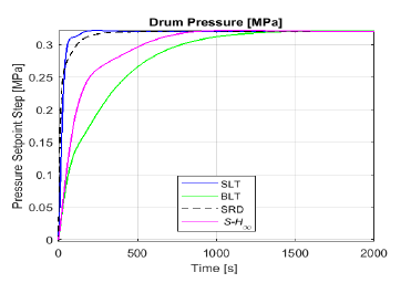Figure 6: Step response of drum pressure for each method

The former picture changes in Figure 6, where SLT still holds the fastest tracking, but after detuning, BLT results too conservative. It is worth noting that SRD performs closely to SLT.

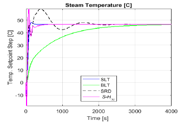Figure 7: Step response of steam temperature for each method Temperature tracking in Figure 7 reveals that SH_∞ method reaches the setpoint first. Even though this response is fast, it is also under-damped, and the settling time of S-H_∞ and SLT turn out to be nearly the same. Besides, SRD shows a under-damped, slow response, while BLT presents a very slow, over-damped evolution.

5.4. Controller Output

As established in Section 2.2, there are control constraints that must be satisfied. Such verification is crucial, as most design methods in this work do not consider any kind of constraint, with the sole exception of S-H_∞. In this regard, even when S-H_∞ consider design constraints, it provides only indirect ways to apply the restrictions established in (13). For instance, fuel flow rate may be bounded by limiting control energy or overshoot. As a consequence, there is no guarantee of meeting control limits, so every method must be reviewed.

The following figures display a selection of controller outputs after a setpoint step change. For these figures, upper and lower limits from (13) are easily visualized by parallel red lines. Particularly, Figure 8 presents feed water flow rate following a 10% increase of level setpoint. It is clear that SLT control output exceeds the imposed upper limit. This is, in fact, consistent with que quick response of SLT observed in Section 5.3.

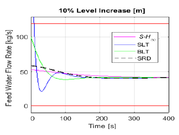Figure 8: Control output of feed water flow rate for each tuning method, following a 10% increase in level setpoint

An similar behavior is presented in Figure 9, where the evolution of fuel flow rate is shown for a 10% increase of level setpoint. In this case, SLT surpasses the lower limit imposed, whereas the remainder methods meet the requirements. Once again, this is consistent with the more aggressive control action observed in Section 5.3. It is worth noting that, in practice, these constraints violations lead to completely different dynamic responses, as the control signal is saturated, so is not able to follow the former simulations.

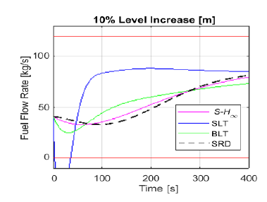Figure 9: Control output of fuel flow rate for each tuning method, following a 10% increase in level setpoint

Figure 10 shows fuel flow rate derivative u˙₂ evolution after a 10% increase of level setpoint. As it can be seen, not only u₂ exceeds its limits, but also the corresponding derivative u˙₂.

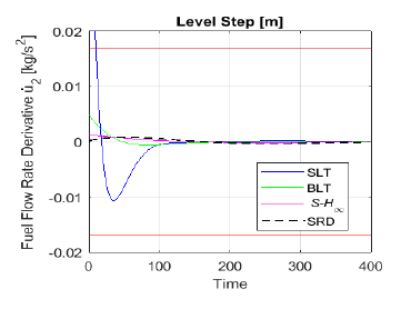Figure 10: Control output of fuel flow rate derivative for each tuning method, following a 10% increase in level setpoint

Finally, Figure 11 displays fuel flow rate derivative u˙₂ following a 5% increase of pressure setpoint. As previously indicated, SLT response does not meet constraint limits. Surprisingly, SLT is the only design method that violates constraints, even though neither BLT nor SRD has any kind of consideration for design restrictions. A possible explanation is that both BLT and SRD yield more robust designs, and this prevents from having excessive control actions.

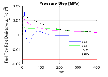Figure 11: Control output of fuel flow rate derivative for each tuning method, following a 5% increase in pressure setpoint

6. Conclusion

Preliminary analysis of the plant presents some issues which may affect control design. Particularly, controller output must meet a set of constraints. Regarding the mathematical model, there are pure integrators in some matrix elements, which has an impact on stability. Also, inverse response may occur due to the system is non minimum phase. Finally, even though interactions among loops are not strong, they are not negligible either.

Four tuning methods were applied using the same control structure, namely, PI architecture. Taking into account integral performance and dynamic response, SLT stands as the best design at a first glance. This prospect is attractive since it is the most simple approach. However, this design fails to meet control out-put limits. For this reason, SLT turns out to be misleading and must be discarded as a valid solution. By contrast, BLT technique, which comes from detuning SLT parameters, achieves an excessive robustness. This is confirmed with the slow dynamic responses of Figures 6 and 7. In this way, only SRD and S-H_∞ provide satisfactory designs. These two techniques imply similar tuning effort, being SRD slightly more straightforward because it has less possible tuning goals. Nonetheless, integral performance shows that S-H_∞ outperforms SRD regarding setpoint tracking, as ITAE index differs by an order of magnitude from that of SRD, while ISE indexes stay on the same order of magnitude for both techniques. In addition, S-H_∞ offers a superior disturbance rejection than SRD for ISE as well as ITAE indexes.

Another reason for which S-H_∞ turns out to be a convincing option is that this method guarantees internal stability. Even though no stability issues were presented for this plant, it remains a desirable feature.

To sum up, S-H_∞ yields the best design, justifying the additional computational cost and tuning effort that it requires. Another useful conclusion is that it is easy to misjudge the best design performance without a careful analysis. Finally, it is worthwhile noting the importance of considering constraints along the design process, in order to avoid further revisions. In fact, operative constraints are ubiquitous in every practical system.

Conflict of Interest

The authors declare no conflict of interest.

1. W.L. Luyben. Simple method for tuning siso controllers inmultivariable systems. Ind. Eng. Chem. Process Des., 25:654–660, 1986.
2. P. Apkarian and D. Noll. Nonsmooth H1-synthesis. IEEE Transactions of Automatic Control, 51:229–244, 2006.
3. P. Apkarian and D. Noll. Structured H1-control of infinite dimensional systems. International Journal of Robust and Nonlinear Control, 2018.
4. E. Adam. Instrumentaci´on y Control de Procesos: Notas de Clase. Universidad Nacional del Litoral, 2011.
5. W. Tan and H. J. Marquez. Stabilizer design for industrial cogeneration systems. Control Engineering Practice, 10:615–624, 2002.
6. E.J. Adam and C. J. Valsecchi. Multiloop control applied to integrator mimo processes. XXII Interamerican Confederation of Chemical Engineering, page 18, 2006.
7. D. Gu, P. Petkov, and M. Konstantinov. Robust Control Design with Matlab. Springer, 2005.
8. J. M. Maciejowski. Multivariable Feedback Design. Addison- Wesley, 1989.
9. E. Bristol. On a new measure of interaction for multivariable process control. IEEE Transactions on Automatic Control, 11:133–134, 1966.
10. W. Hu, W. Cai, and G. Xiao. Relative gain array for mimo processes containing integrators and/or differentiators. 11^th International Conference on Control Automation Robotics and Vision, 1:6, 2010.
11. S. Skogestad and I. Postlethwaite. Multivariable Feedback Control – Analysis and Design. Wiley, 1996.
12. K. Zhou and J. C. Doyle. Essentials of Robust Control. Prentice Hall, 1999.
13. D.Q. Mayne. The design of linear multivariable systems. Automatica, 9:201–207, 1973.
14. G. Zames. Feedback and optimal sensitivity: Model reference transformations, multiplicative seminorms, and approximate inverses. IEEE Transactions on Automatic Control IEEE, 26:301–320, 1981.

(Click Here)

(Click Here)