1. Introduction

Accidents and disasters such as building collapses, fires, earthquakes, and floods are responsible for massive loss of life. According to an interview survey about the Great Hanshin-Awaji Earthquake (also known as the Kobe Earthquake) of 1995, the most important contribution to rescue activities following such an event is rapid information gathering. Therefore, search robots are attracting attention as rapid means of gathering such information. In late years, a lot of researchers have been developed varied robots, and there has been remarkable progress in unmanned aerial and ground vehicles. For example, to save the electric power and to extend the inspection time on aged bridges, a UAV with a magnetic adsorption device was proposed and developed by Akhara et al [1]. The quadrotor helicopter based UAV has an adsorption device using electro permanent magnets (EPM). And two cameras are set on the camera arms to carry out the close visual inspection.

Oliver et al. reported about a quadrotor helicopter with a tilt mechanism in [2]. The proposed quadrotor helicopter can fly horizontally while maintaining a steady attitude to conduct aerial inspection with stable condition. The development of unmanned multirotor helicopters has led to expand applications, such as (i) inspecting aerial power lines for maintenance, (ii) constructing platforms with which to rescue people, and (iii) undertaking construction on inaccessible areas [3]. On the ground, walking robots are able to cross irregular ground that is impossible to wheeled and crawler robots, leading to the development of experimental dynamic walking robot[4], [5]. Also, unmanned vehicles have been developed that can both terrestrial locomote and fly in the air. This is because in search scenarios it is often necessary to both fly quickly over extended areas and search carefully on the ground. Pratt and Liang developed the dynamic underactuated flying–walking (DUCK) robot, which combines a quadcopter helicopter with passive-dynamic legs to create a various system that can fly and walk [6].

To coordinate walking and flying abilities, in [7], the authors designed and constructed the legged air vehicle shown in Fig. 1. The frame, legs and the body are constructed from pipes and plates of carbon-fiber reinforced polymer for high stiffness and low weight. Two brushless motor and propellers are equipped as the thruster. And four legs composed of servomotors and parallel link mechanisms are used for walking and controlling the attitude.

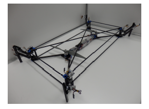Figure 1: A prototype of the proposed legged aerial vehicle.

Table 1: Specifications of the legged aerial vehicle.

                              Length [mm]       702–870

                               Width [mm]       400–560

Height [mm] 120–200 Weight [g] 830

The flight attitude of the robot is controlled by changing of the center of gravity (CoG) caused by motion of the legs. The control using CoG can reduce the number of actuators than the sum of those required for controlling a quadrupedal robot and a tandem-rotor helicopter individually. With respect to flight control using change of CoG, there is a quadrotor helicopter controlled by an inverted pendulum. Miwa developed the quadrotor helicopter equipped an inverted pendulum on top of the body, and achieved control the attitude by using the tilt angle of the pendulum [8]. The present paper describes construction of mathematical models of the legs, rotors, and development of attitude control system based on them to simulate the motion of the robot in the air. And the behavior of the robot in the air is simulated using the constructed model and a physical model constructed in ADAMS. ADAMS is an analysis software to simulate the behavior of moving parts and distribution of loads and forces to the whole robot without solving the equations of motion analytically.

2. Model of a Leg and Parameter Identification

The inputs of the physical model constructed by

ADAMS are forces such as the driving torques and thrusts of the legs and rotors, but the inputs of the actuator are voltage signals that depend on reference profiles of the leg angles and rotor speeds. Therefore, this section presents a mathematical model of the legs and identifies the relevant parameter values. The model is built to clarify the relation between the servomotor input and the drive torque. Figure 2 shows the servomotors for driving links around a roll axis and a yaw axis, and a parallel link mechanism of links.

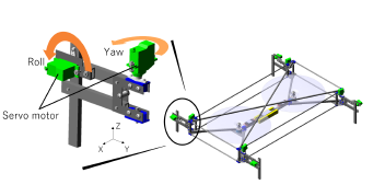Figure 2: Servomotors and a parallel link mechanism of the leg

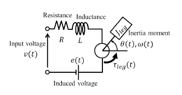Figure 3: Electro-mechanical model of the direct current (DC) motor in one of the servomotors, including the effect of the moment of inertia, friction, and gravity.

We assumed that the leg could be modeled as a servomotor model that includes the influences of the moment of inertia, friction, and weight of the leg about each axis. Figure 3 shows the model of a direct current (DC) motor in servomotors. The driving torque of a the leg τ_leg(t) driving the leg is presented as the sum of the torques τ_m(t), τ_f (ω(t)), and τ_g(θ(t)). Here, τ_m(t), τ_f (ω(t)), and τ_g(θ(t)) are torque of the servomotor, friction, and gravity, respectively. Thus

where t, ω(t) and θ(t) are time, the angular velocity and angle of the leg from a chosen reference.

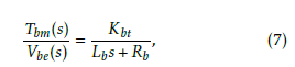
The transfer function from the differential voltage to the motor v_e(t)(= v(t) − e(t)) to servomotor torque τ_m(t) the [9] is expressed as

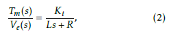by using the coil inductance L, the motor resistance R and the torque coefficient K_t. And T_m(s) and V_e(s) are the Laplace transforms of τ_m(t) and v_e(t).

The friction torque τ_f (ω(t)), which is a function of the angular velocity ω(t) of the leg, is given below[10]: τ_f (ω(t))

where τ_s is the static friction torque, τ_act(t) is the sum of τ_m(t) and the gravity torque τ_g(t), and a₁, a₂, and a₃ (a₁ + a₂ = τ_s) are positive. Therefore, the Laplace transforms of the leg angle Θ(s) is presented as

Hrere, T_leg and J_leg are the Laplace transforms of τ_leg(t) and the moment of inertia of links and servomotors.

The servomotor controller is taken to be a proportional–derivative (PD) controller [9] as given by

where K_sp and K_sd are the proportional gain and differential gain, respectively. θ_ref (t) is the reference input of the leg angle.

In generally servomotors are controlled by PD controller to earn rapid response. The controller does not include an integral (I) controller. Therefore the measurement angle has slight angle error to the reference as shown in Figs. 4 and 5. The drive angle of a DC motor in the servomotor is measured by an installed potentiometer or a rotary encoder. Measured value has some electric noise, however, the noise does not cause terrible error because these signal passes a low pass filter. The unknown parameters A, B and C are estimated using the Levenberg–Marquardt method which is one of the iterative technique that locates the minimum of a function that is expressed as the sum of squares of nonlinear functions. To identify the parameters, the response of the leg about each axis was measured by using following the three steps below:

1. Attach two light-emitting diodes (LEDs) to the leg (see Figs. 4 and 5).
2. Record the motion of the leg to a video (30 fps) andthe reference angle to a micro computer.
3. Apply image processing to each frame of the videoto calculate the coordinates of each LED.
4. From those coordinates, calculate the angle of theleg for each frame.

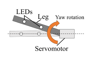Figure 4: Leg motion in angle measurement experiment for the yaw rotation using LEDs.

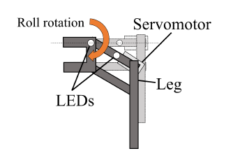Figure 5: Leg motion in angle measurement experiment for the roll rotation using LEDs.

We determine the parameter values by minimizing the squared difference between the measurements and the simulation values using the models shown in Figs 4 and 5. Here, the simulation frequency was 1 kHz. Table 2 lists the identified parameter values, and Figs. 6 and 7 show the simulation results for each axis accompanied by the respective measurements. These simulation results shows that the behavior of the leg model is close to the measured behavior.

Table 2: Result of Parameter Identification Symbol  Identified value

Kt	0.2016
a3	0.035
Ksp	0.912
Ksd	0.005
a2	0.070

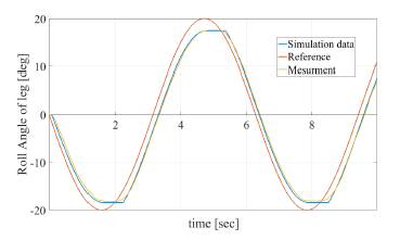Figure 6: Simulation results of roll angle of the leg. Blue line is simulation result using identified parameters. Mearment data is measured roll angle through the experiment shown in Fig. 5.

3. Model of Rotor

We explain the model of a rotor composed of a propeller and a brushless motor assumed as a DC motor in this section. The brushless motor is assumed as a DC motor. Thus, as with Eq. (2), the transfer function from the differential voltage to the motor torque is given as

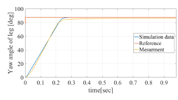Figure 7: Simulation results of roll angle of the leg. Blue line is simulation result using identified parameters. Mermen data is measured yaw angle through the experiment shown in Fig. 4.

V_be(s)   L_bs +R_b where each variable corresponds to the respective one in Eq. (2).

The thrust T (t) generated by the propeller and the counter-torque τ_c(t) acting on the propeller due to the air are known to be proportional to the square of the rotor velocity in the steady state. Therefore, T (t) and τ_c(t) are calculated using approximation curves based on the data sheet of the propeller on the manufacturer APC’s web site [11]. Those thrust and torque are given as

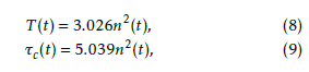where n(t) is the rotation velocity in units of revolutions per minute (rpm); Eqs. (8) and (9) are plotted in Figs. 8 and 9, respectively. Moreover, the relationship between the rotation velocity ψ(^˙t) in units of radians per second (rad/s) and the torque τ_p(t)(= τ_bm(t) − τ_c(t))

where J_p is the inertia torque of the propeller, and Ψ˙ (s) and T_p(s) are the Laplace transforms of ψ˙(t) and τ_p(t). The response of the rotor is simulated based on these equations.

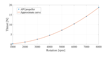Figure 8: Thrust data from manufacturer’s site [11] and approximation curve.

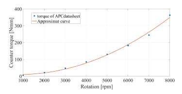Figure 9: Counter-torque data from manufacturer’s site [11] and approximation curve.

4. Attitude Control using the Leg Motion

4.1. Modeling of CoG and Leg Angles

To develop a control system for CoG control, we clarify relation between the CoG and the leg angles. The variables and link names are defined as shown in Figs. 10 and 11. The masses of links B, U, L, and F are m_b, m_u, m_l, and m_f , respectively, and those of the leg and the vehicle are m and M, respectively. The matrix θ ∈ _R^2×4 of legs angles is defined as

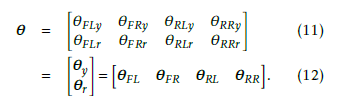
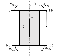Figure 10: Definition of leg angles around the yaw axis.

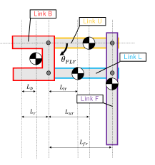Figure 11: Definition of angles and link parameters on the front-left (FL) leg.

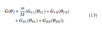
By the definitions, the robot CoG G(θ) = {G_X,G_Y }^T is expressed following Eq. (13) in terms of the various leg CoGs, namely G_FL(θ_FL), G_FR(θ_FR), G_RL(θ_RL), and GRR(θRR):

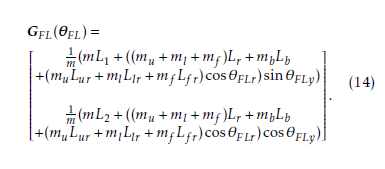
Each leg CoG is determined from the respective leg angle. The CoG of the front-left leg (FL) is given by

The vehicle CoG is calculated from Eqs. (13) and (14) and the various leg angles.

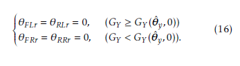
However, the reference leg angles cannot be determined uniquely from the reference CoG because of θ ∈ _R^2×4 and G ∈ _R². Assuming that leg motion around the yaw axis and roll axis cause movement of the CoG along X and Y axis each, the conditions for the leg yaw angles are

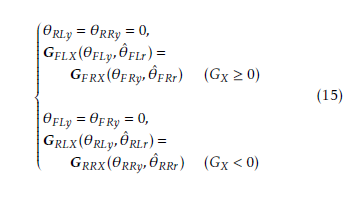by using the estimated leg angle matrix θˆ. And those

Also, when G_Y ≥ G_Y (θˆ_y,0) is satisfied, the additional

conditions are

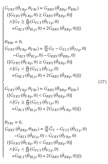When another condition is to be satisfied, the additional conditions are given with suffixes representing the right and left sides of the robot. Thus, the reference leg angles are determined based on the relation between a leg CoG and this angle in the conditions.

4.2. Calculation of Reference Position of CoG

The reference CoG for attitude control is calculated from the error in the attitude angle trajectory. In the first step, the pitch-roll-yaw torque around the CoG acting the entire aircraft τ_CoG(t) = {τ_p(t),τ_r(t),τ_y(t)} is calculated from a PD controller shown below:

by using the pitch-roll-yaw (φ_p(t),φ_r(t),φ_y(t)), φ(t) ∈ R³, and their reference φ(t)_ref ∈ _R³. Where K_p, K_d ∈ _R³ are the proportional gain and differential gain, ∗˙ is differential of the ∗, and ◦ is Hadamard product. In the second step, the thrusts and the center of thrust (CoT), which is the position of the torque around the CoG balancing caused by the thrust, is estimated from the input values using the rotor model. The estimated thrusts and CoT are represented by Tˆ(t) = {Tˆ₁(t),Tˆ₂(t)}^T and CoTˆ (t) = {CoTˆ _X(t),CoTˆ _Y (t)}^T , respectively. The final step determines the reference CoG G_ref (t) = {X_ref ,Y_ref }^T from the torque, the thrust, and the CoT given by the first and second steps by the following equation:

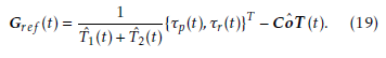Meanwhile, reference rotor speed is determined by τ_y(t) and the reference of the sum of the thrusts is determined using Eqs. (10) and (9).

5. Attitude Control Simulation

The motion of the robot was simulated based on the physical model constructed by ADAMS and the control system constructed by a numerical analysis software MATLAB. Simulation parameters are the same values to those of the prototype. The sampling frequency of simulations was 1 kHz. And Table 4 shows reference angles in the simulations.

Figures 12 and 13 show the pitch angle for simulation pattern 1 and the roll angle for simulation pattern 2. Fig. 14 shows the result of the yaw angle for simulation pattern 3. Results in Figs. 12, 13, and 14 corresponded with the respective reference lines, and showed that the developed control system was effective through the simulations.

Figures 15 – 19 show detail of the pitch, the roll and the yaw angle in several reference angles including large reference. When the pitch reference is 20 deg shown in Fig. 15, the pitch angle follows the reference rapidly. although the roll angle changs like a sine wave in this simulation,the control paformance is enough effective because the range is very narrow between -0.5 and 0.5deg. In case of the roll reference is 20 deg, the pitch angle did almost not change as shown in Fig. 16. The reason that the change of the pitch angle in Fig. 16 is smaller than the change of the roll in Fig. 15, is difference of the moment of inertia and variable range of the CoG

The moment of inertia of the robot around the pitch axis is larger than one around the roll axis. And the range of change of CoG to control the pitch angle is also wider than one of the roll control. Therefore the stability of pitch angle is better than the performance of the roll angle.

The effect appeared in the yaw angle too. However the change of except for target angle is very small, and these results showed validness of the developed controller. Especially the roll control worked in large reference 25 deg (Fig. 17) which was enough for flight control. The yaw control also generated slight change in other axes when reference are low (Fig. 18) and high (Fig. 19).

Table 3: Proportional–derivative (PD) controller gains

	Kp	Kd
Pitch	1.0	0.5
Roll	2.0	1.3
Yaw	0.1	0.55

Table 4: Reference of attitude angles in control simulations

	Pitch [deg]	Roll [deg]	Yaw [deg]
Pattern 1	5.0	0.0	0.0
Pattern 2	0.0	5.0	0.0
Pattern 3	0.0	0.0	20.0
Pattern 4	20.0	0.0	0.0
Pattern 5	0.0	20.0	0.0
Pattern 6	0.0	25.0	0.0
Pattern 7	0.0	0.0	10.0
Pattern 8	0.0	0.0	30.0

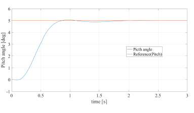Figure 12: Step response of pitch-angle controller (pattern 1, reference pitch:5.0, roll:0.0, yaw:0.0).

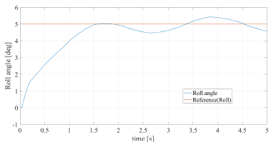Figure 13: Step response of roll-angle controller (pattern 2, reference pitch:0.0, roll:5.0, yaw:0.0).

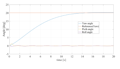Figure 14: Step response of yaw-angle controller (pattern 3, reference pitch:0.0, roll:0.0, yaw:20.0)

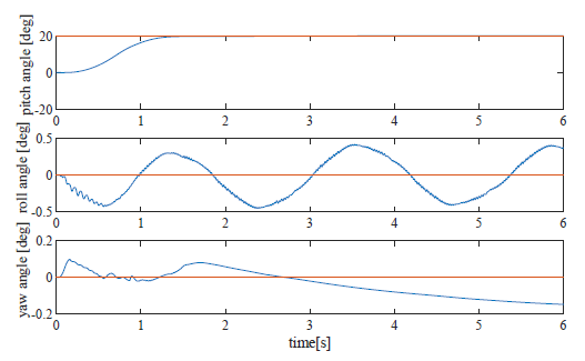Figure 15: Response of three axes (pattern 4, reference pitch:20.0, roll:0.0, yaw:0.0)

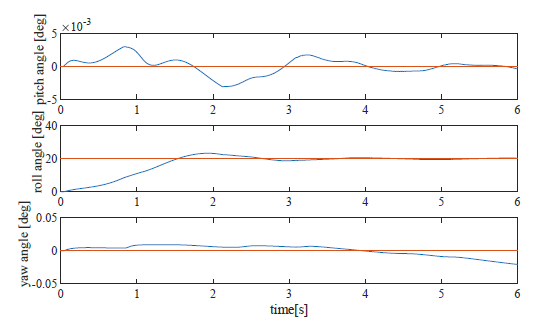Figure 16: Response of three axes (pattern 5, reference pitch:0.0, roll:20.0, yaw:0.0)

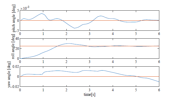Figure 17: Response of three axes (pattern 6, reference pitch:0.0, roll:25.0, yaw:0.0)

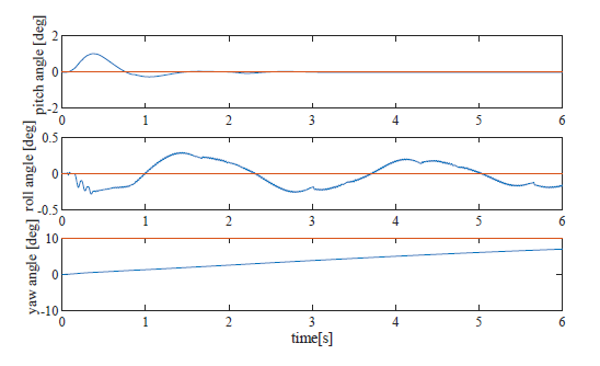Figure 18: Response of three axes (pattern 7, reference pitch:0.0, roll:0.0, yaw:10.0)

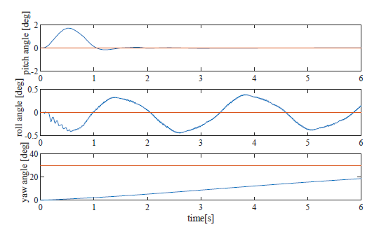Figure 19: Response of three axes (pattern 8, reference pitch:0.0, roll:0.0, yaw:30.0)

6. Conclusions

The paper has described modeling of the leg and the rotor including the propeller, and a control method using the change of the CoG caused by the leg motion. Flight attitude was simulated for some reference angles by the developed control system. These simulation results shows that (i) response of the leg model corresponded to the experimental data and (ii) the attitude angles of the robot could follow their references using the attitude control system. Moreover the difference of moment of inertia and range of CoG in each axis appeared in the results, it was shown that the constructed model could reflect the characteristic of the robot. However, the results also showed that the transient response is not yet fast enough. Particularly convergence of the yaw angle for the yaw reference was slow, even though the yaw angle could follow the reference at last. Future work will involve implementing the control system on the developed legged aerial robot to evaluate the control performance.

1.  S. Akahori, Y. Higashi, A. Masuda, Development of an Aerial Inspection Robot with EPM and Camera Arm for Steel Structures, Proceedings of the International Conference, pp. 3546-3549, 2016.
2.  Russell Oliver, Sui Yang Khoo, Michael Norton, Scott Adams, Abbas Kouzani, Development of a Single Axis Tilting Quadcopter, Proceedings of the Proceedings of the International Conference, pp. 1851-1854, 2016.
3.  A.E Jimenez-Cano, J. Braga, G. Heredia, A. Ollero, Aerial Manipulator for Structure Inspection by Contact from the Underside, Proceedings of the International Conference on Intelligent Robots and Systems, pp. 1879-1884, 2015.
4.  S. Kitano, S. Hirose, G. Endo, Design and Development of Quadruped Robot TITAN-XIII, Journal of Japan Society for Design Engineering, volume 51, number 12,pp. 875-884, 2016.
5.  M. Raibert, K. Blankespoor, N. Gabriel, R. Playter, BigDog, the Rough – Terrain Quadruped Robot, Proceedings of the 17th IFAC World Congress, Vol, 41, Issue 2, pp. 10822-10825, 2008.
6.  C. J. Pratt and K. K. Leang, Dynamic Underactuated Flying- Walking (DUCK) Robot, Proceedings of IEEE International Conference on Robotics and Automation (ICRA), pp. 3267- 3274, 2016.
7.  Y. Higashi and R. Okada, Suggestion of Legged Air Vehicle for Locomotion on ground and in air, Proceedings of the 8th International Conference on Intelligent Unmanned Systems, pp. 228-231, 2012.
8.  M. Miwa, S. Kunou, S. Uemura, A. Imamura, H. Niimi, Attitude Control of Quad-Rotor Helicopter with COG Shift, Journal of JSEM, vol. 13, Special Issue, pp. s102-s107, 2013.
9.  Ishikawa M., Kitayoshi R., Wada T., Maruta I., Sughie S., Modeling of R/C Servo Motor and Application to Underactuated Mechanical Systems, Transactions of the Society of Instrument and Control Engineers Vol.46, No.4, pp. 237-244, 2010.
10.  B.Armstrong, Friction:Experimental Determination,Modeling and Compensation, Proceedings of the 1988 IEEE International Conference on Robotics and Automation, p.1422, 1988.
11.  J. J. More, The Levenberg–Marquardt algorithm: Implementation and theory Proceedings of Conference on numerical analysis, CONF-770636-1, 1997.
12.  APC Propeller Performance Data, http://www.apcprop.com/ v/downloads/PERFILES WEB/datalist.asp, 2017/01/27

(Click Here)

(Click Here)