1. Introduction

This paper is an extension of works originally presented in ICCABS 2017 (International Conference on Computational Advances in Bio and Medical Sciences) [1] and CSCI 2017 (International Conference on Computational Science and Computational Intelligence) [2].

Almost every cell in an organism’s body contain the same genetic information and series of genes, what makes cells different is which genes are expressed at any time. Gene expression is what makes a blood cell different from a liver cell and a normal healthy cell from an abnormal one (like a cancer cell) [3]. Gene expression process has two steps, transcription and translation. Transcription means a particular part of DNA is encoded into messenger RNA (mRNA) and in translation, mRNA is decoded to build a protein that contains a specific series of amino acids. We can measure the gene expression level by measuring the amount of mRNA inside the cell. Each step of the process is regulated by control points that determine the presence and the amount of proteins in any specific cell [4]. Usually a group of genes work accordingly to manage every simple or complex process that control the structure and actions of the cells. This means that group of genes must work together in order to control structure and actions of cells [5]. Knowing this, we can conclude that the gene expression levels should be highly correlated so if the data has missing values, we might be able to predict them based on the correlation between genes.

Recently scientists have the opportunity to find the association between genes and diseases using some methods. Examples of this methods are RNA sequencing, northern blotting, western blotting, DNA microarray, fluorescent in situ hybridization and reporter gene. However the costs of measuring gene expression levels are extremely high and also the complete process needs a huge amount of time [6] which makes it difficult to measure and access this information. Also gene expression data usually suffers from missing values. This can happen due to some reasons like failures in hybridization, noise in data and also data corruption. Missing values in gene expression data can negatively affect gene disease studies [7]. Since due to the huge amount of time and money needed for repeating the measurements, an alternative way is to use computational methods which can be employed to predict the missing values and recover the dataset. So there is a high demand for novel techniques to find the missing values.

The first step to make our model is to store gene expression data in matrices where each row is a different gene, each column is a different disease and the entries of the matrix are the gene expression values (mRNA measurements) of corresponding rows and columns [8]. Based on this model we can assume that people with similar diseases show similar expression patterns so the gene expression data matrix must be highly overdetermined and significantly low rank [9].

1.1.  Recommendation system

Recommendation systems rely on information filtering in order to deal with data overload by filtering necessary information which is significantly less than total data of users’ preferences, interests or observations about an item. Recommender systems have the ability to recommend a new movie to a specific user based on his/her previous preferences [10]. Recently different designs for recommendation systems have been proposed which are based on one of these methods: collaborative filtering method [11], content-based filtering method [12] and hybrid filtering method [13].

1.2.  Collaborative Filtering Method

Collaborative filtering method recommends item to users by recognizing users with similar tastes. It combines other ratings in order to recommend new items to each specific user. Collaborative filtering techniques are categorized into two groups: model-based technique and memory-based technique. The main goal for model based method is making a model and extract the necessary part of the data matrix so there is no need to use the entire dataset in order to make predictions [14]. Memory based technique uses previously collected data in order to predict the missing ratings and they use the entire user-item database. The common memory based method is based on nearest neighbors and uses a distance measure metric to find the neighbors [15]. This is also called neighborhood based approach which similar users are grouped together based on their interests [16].

Netflix is an example of recommendation systems that can benefit from collaborative filtering technique. For the Netflix example, the proposed model contains a  matrix.  Each row of the matrix corresponds to a different user and each column corresponds to a different movie and the entries of the matrix are the ratings users gave to the movies. The data matrix is very sparse because most users usually tend to rate a very small fraction of the movies, the matrix is very sparse. So the goal is to find the hidden pattern and predict the missing values in order to make a recommendation to users for the movies that they have not watched yet.

1.3.  Low Rank Matrix Completion

Matrix completion (MC) involves recovering an incomplete matrix where only a small fraction of its entries are known which is significantly smaller than the total size of the matrix. Low rank MC problem can be seen in different practical contexts such as image processing [17], machine learning [18] and bioinformatics [19]. To solve this problem, we should find the lowest rank matrix which is consistent with the known values of the incomplete matrix.

Here  is the incomplete matrix that we want to reconstruct,  shows the known values such that  if  is known.  is the orthogonal projection matrix where: Because the rank minimization problem is NP-hard, this   problem can be remodeled as minimizing trace norm or nuclear norm. Nuclear norm is the sum of singular values of the given matrix [20]. The reason is that a rank  matrix with has exactly  singular values which are greater than zero. The nuclear norm of matrix

   is the a^th singular value (nonzero) of matrix  and  is the rank of matrix .

The advantage of using nuclear norm over minimizing the rank is that its optimum point can be calculated efficiently and it is convex.

1.4.  Robust PCA method (RPCA)

One problem with gene expression datasets is the presence of noise in expression measurements. This happens because of some reasons like different degrees of uniformity, small spots, process errors and also inconsistency in hybridization.

For the aim of showing the most variability of the data for a noise free dataset, we can easily perform PCA using SVD (singular value decomposition). In the presence of noise we can use RPCA in order to reconstruct a low rank matrix and find the sparse noise. Assume that our data matrix

Where is the underlying low rank matrix and  is a sparse matrix capturing noise. Because the number of unknowns to infer for  is considerably higher than known values in , this problem is overdetermined. So we need to use tractable convex optimization

Where  is the -norm of and is a parameter.  This should work even in the situations when the rank of  is not low rank (when rank is equal to the dimension of the matrix). For RPCA method to work efficiently, we need to know the location of the non-zero entries in matrix . Problem can be solved at a cost not so much higher than classical PCA [21].  One of the methods that can be employed here is the Alternating Direction Method of Multipliers (ADMM) that we will summarize in the next section.

1.5.  The ADMM method

The ADMM method is a powerful method because it mixes two methods of multipliers and dual ascent. The algorithm solves the problems

Where  are both convex. The optimal value for the problem above is defined as:

Where  is the Lagrangian multiplier and  is a parameter. ADMM method consists of the multiple iterations

The algorithm consists of multiple steps:

1. An a-minimizing step
2. A b-minimizing step and
3. A variable update.

In the last step (variable update step) the step size is equal to the  (the augmented Lagrangian parameter).

2. Methods

2.1.  Correlation based Matrix Completion method

The main goal of the correlation based matrix completion method (CMC) is finding correlation between genes (neighbors). To predict a value for a missing entries, we need to consider all other subjects’ expression values. If a gene is more similar to the one with a missing value, its expression value has more impact on the predicted value. For finding correlation between genes, we will use Pearson correlation coefficient (PCC), Euclidean distance (ED) and Cosine similarity (CS).

Pearson Correlation Coefficient

PCC is a common measure of linear dependency between two variables. The PCC can take any value from 1- (means negative association) to 1 (means positive association) with 0 indicating orthogonality. The PCC can be calculated by:

Euclidean Distance

Euclidean distance (ED) is a metric that if x and y have zero distance, then x = y holds. ED between two points (x and y) can be calculated

Cosine Similarity

The Cosine Similarity (CS) is a metric of the cosine of the angle between two vectors. This is a measurement of orientation instead of magnitude. Like PCC, CS can take any value from 1- (means negative association) to 1 (means positive association) with 0 indicating orthogonality. The CS value can be calculated as shown below:

CMC Approach

Here we explain how CMC approach works in order to find missing values in partially known matrices. Let us assume that we have a complete (means all the entries are known) low rank matrix . Now if we randomly remove some of the values, the problem becomes how to find missing values in a way that there was not a huge difference between the original values and the predictions. We will use PCC, ED and CS in order to reconstruct matrix  and the reconstructed matrices when using each of the aforementioned similarity metrics are Y_P, Y_E and Y_C respectively.

This is how the CMC method works:

• First a PCC, an ED and a CS value should be calculated for each pair of the genes.
• When there is a missing value, we need to calculate the mean of all known entries in that column weighted by how correlated they are (based on their PCC, ED and CS values).
• Finally we will measure the accuracy of each method by calculating the error between the reconstructed matrices and the original matrix.

For finding a missing value at Y (m,n)

Algorithm 1 shows the pseudo code for correlation based matrix completion approach.

Algorithm 1. Correlation based matrix completion approach

Input: Y, ω

For row m of Y:

    For row n of Y:

        If m != n :

            Find PCC (m,n)

            Find ED(m,n)

            Find CS (m,n)

For row m of Y:

    For row r of Y:

        If (m,r) in ω:

            Y_p(m,r) = Y(m,r)

            Y_e(m,r) = Y(m,r)

            Y_c(m,r) = Y(m,r)

        Else if (m,r) not in ω:

            Y_p(m,r) = 0

            Y_e(m,r) = 0

            Y_c(m,r) = 0

            x = 0

            for row p of Y:

                if (p,n) in ω:

                    Y_p(m,r) += Y_p(r,n) *PCC(m,p)

                    Y_e(m,r) += Y_e(r,n) * ED(m,p)

                    Y_c(m,r) += Y_c(r,n) * CS(m,p)

                    x++

           Y_p(m,r) /= x

           Y_e(m,r) /= x

           Y_c(m,r) /= x

output: Y_P, Y_E, Y_C

2.2.  Convex Optimization Formulation of RPCA method

Updating matrix Y

For solving above problem, we can use a soft thresholding operation from [22]. So the problem would become:

Where  is the step size which decreases the singular values of matrix A and the shrink is a soft-thresholding operator and can be defined as:

Where  is the singular values and  is the left is the right singular vectors of matrix M.

Updating matrix S:

After updating Y, we can update S through:

To solve the above problem, we can use a shrinkage operator:

Where  is the shrinkage operator discussed in [23] and can be calculated by: We can assume that entries in matrix S that represent missing values are equal to zero.

Updating m:

After updating Y and S, we can update m by:

Algorithm 2 shows the pseudo code for solving RPCA problem using ADMM.

Algorithm 2. Solving RPCA problem using ADMM

Input: E, ρ, λ, ε

While ║E – Y^k – S^k║_F > ε:

    Updating matrix Y:

    Y^k = arg_Y min Lρ(Y^k-1, S^k-1, m^k-1)

    Y^k = shrink ((E – S^k-1 + ),ρ^-1)

        (U,S,V) = SVD (E – S^k-1 + )

        For singular values σ in S:

            If σ <  :

                σ = 0

        Y^k = U S V^T

       Updating matrix S:

    S^k+1 = arg_S min Lρ(Y^k+1, S^k, m^k)

    for row p of S:

        for column r of S:

            if (p,r) in ω:

                S_pr = H  (E – Y^k + )

            else:

                S_pr = 0

    Updating m:

    m^k  = m^k-1 + ρ(E – S^k – Y^k)

output: Y^k and S^k

3. Competitive methods

3.1.  K-nearest Neighbors method

K-nearest neighbors (KNN) is one of the most essential classification algorithms in machine learning. It can be widely used in real-life scenarios since it does not make any assumption about the distribution of the data. The model representation for KNN is the entire dataset and it can make predictions using the training data set directly. When there is a missing value, prediction can be made by searching through the dataset for the K most similar neighbors and the result is the weighted average of those neighbors [24]. To determine which K neighbors are the most similar ones, a distance measure should be used and Euclidean distance is the most popular one for real-valued variables.

3.2.  Nuclear Norm Minimization

There are various numerical methods available to solve. The important problem is that because of the high dimensionality aspect of biological data, many numerical methods fail to solve the problem efficiently. Kapur et al. [25] used a method called soft thresholding operator which can scale well on large datasets. So the problem would become:

Where  is the Frobenius norm and  is the thresholding parameter and it should be greater than 0. We can reconstruct the expression matrix iteratively so the k^th iteration would be:

Where shrink is the soft thresholding operator [22]. The parameter  is the step size and the parameter minimizes the rank by decreasing the singular values. The shrink operator is defined by:

Where  is the left and is the right singular vectors of data matrix  In each iteration the SVD of matrix is calculated and those singular values that are smaller than parameter, will be set to zero. The new matrix will be reconstructed. Algorithm 3 shows the pseudo code for this method.

Algorithm 3. Nuclear Norm Minimization Problem

Input: Y, ω, ε

δ = 1.2 *(mn)/│ω│

τ = 5 *(mn)^0.5

Shrink(Y, τ)

    (U,S,V) = SVD (Y)

    For singular values σ in S:

        If σ < τ:

            σ = 0

    M = U S V^T

Minimize(Y, ω)

    For row a of Y:

        For column b of Y:

            If (a,b) in ω:

                Rω (Y) = Y

            Else:

                Rω (Y) = 0

    M⁰ = 0

    k = 1

    while Rω (Y^k – X)║_F / Rω (X)║_F < ε:

        Y^k = shrink (Y^k-1, τ)

        M^k = M^k-1 + Rω (X – Y^k)

        k++

output: X^k

3.3.  Singular Value Thresholding Algorithm (SVT)

This approach considers using a Robust PCA approach in order to reconstruct a low rank matrix from noisy measurements Where:

• is the noisy dataset.
• is the low rank matrix.
•  is the noise and it assumed that it only affect a fraction of the data (E is sparse).
•  is a scalar and

    We can apply the Lagrangian multiplier Y in order to replace the equality constraint:

Then in each iteration A, E and Y will be updated by minimizing with respect to A, E and Y. Algorithm 4. Shows the pseudo code for SVT approach where σ is the step size.

Algorithm 4. The SVT Algorithm

Input: τ,D,λ

While not converged:

    (U,S,V) = SVD(Y^k)

    A^k= arg min_x τ║D║_* +  ║D-E^k-1║_F

    E^k= arg min_x τ║D║₁ +  ║D-A^k║_F

      Y^k= Y^k-1 + σ_k (D – A^k – E^k)

End while

output: A = A^k, E = E^k

3.4.  Exact Augmented Lagrangian Multiplier (ELAM)

ELAM method was proposed in [26] and can be used for solving Robust PCA problem. To solve the problem can apply the Lagrangian multiplier as denoted below:

And the Lagrangian function

Algorithm 5. Shows the pseudo code for ELAM method.

Algorithm 5. Exact Augmented Lagrangian Multiplier (ELAM)

Input: matrix D, λ

While not converged:

    (A^k+1, E^k+1) = arg min_A,E L(A,E,Y)

While not converged:

    (U,S,V) = SVD(D – E^k + )

    A^k+1= arg min_x ║D║_* +  ║D-E^k║_F

    E^k+1= arg min_x ║D║₁ +  ║D-A^k+1+ ║_F

End while

      Y^k+1= Y^k + µ^k(D – A^k+1 – E^k+1)

    k++

End while

output: A = A^k+1, E = E^k+1

3.5.  Inexact Augmented Lagrangian Multiplier (ILAM)

ILAM method was proposed in a study by Lin et al [27]. The RPCA problem is closely connected to MC problem so the MC can be formulated

 means that E is zero at indices where the value is known and the augmented Lagrangian  So the ILAM approach can be used for MC problem. The pseudo code for ILAM method is described below.

Algorithm 6. Exact Augmented Lagrangian Multiplier (ELAM)

Input: matrix D, ω, λ

While not converged:

    (A^k, E^k) = arg min_A,E L(E,A,Y)

    (U,S,V) = SVD(D – E^k + )

    A^k= arg min_x ║D║_* +  ║D-E^k-1║_F

    E^k= arg min_x ║D║₁ +  ║D-A^k+ ║_F

    Rω (E) = 0

      Y^k= µ^k(D – E^k– A^k)+ Y^k-1

    k++

End while

output: E = E^k, A = A^k

4. Evaluation

Here we measure the accuracy of different approaches as they apply to biomedical data MC. All of the following experiments were performed using Python 3.6 and Matlab 2016 on an Intel Core i7 PC running Windows 10 with 16GB main memory.

4.1.  Datasets

We downloaded and used 4 gene expression datasets from NCBI (National Center for Biotechnology Information) for our experiments. We used the following gene expression datasets:

Lung Cancer Study

Title of this study is: “Gene expression signature of cigarette smoking and its role in lung adenocarcinoma development and survival”. Scientists found that smoking tobacco is the reason for the most of lung cancer cases, but the exact details of this process is still unknown. In this study Landi et al. used 135 tissue samples of adenocarcinoma and non-involved lung tissue from 3 groups (current, former and never smokers). They found out that expression of some genes is significantly different in smokers and non-smokers. The lung cancer dataset has 22283 rows- and 107 columns [28].

Dementia Study

Title of this study is: “Variations in the progranulin gene affect global gene expression in frontotemporal lobar degeneration”. The symptoms of frontotemporal lobar degeneration is progressive decline in language and function. Despite the excessive research on the reason for this disease, its mechanisms remain unknown. Plotkin et al. isolated postmortem brain samples from normal controls, patients with mutations in progranulin gene and patients without mutations in progranulin gene. The dementia dataset has 22277 rows and 56 columns [29].

Autism Study

Title of this study is: “Autism and increased paternal age related changes in global levels of gene expression regulation”. Autism is a neurodevelopmental disorder and it is the results of transcription factor mutations that can change the gene expression regulation. In this study Alter et al. analyzed gene expression values of 82 subjects with autism and 64 controls. The results showed that autism and increased paternal age can change the gene expression regulation. The Autism dataset has 54613 rows and 146 columns [30].

Bladder Cancer Study

Title of this study is: “Combination of a novel gene expression signature with a clinical nomogram improves the prediction of survival in high-risk bladder cancer”. In this study Riester et al. analyzed data of patients with bladder cancer (n = 93) and measured the gene expression. The bladder cancer dataset has 54675 rows and 93 columns [31].

4.2.  Calculating Error

We used two metrics to determine how accurate the MC algorithm is. So we start with a known matrix   remove a random portion of it (i.e., simulating missing entries), and then try to reconstruct the matrix

Relative Error

Relative error can be used to describe accuracy; specifically, how accurate a measurement is compared to the true value. We use the relative error (RE) which can be calculated as below:

Where is the original matrix and is the reconstructed matrix.

Mean Square Error

We will also use mean squared error (MSE) to measure the accuracy of the different approaches. We can find MSE by calculating the mean of the squares of the deviations, which is the difference between the original and the prediction. The MSE between and  is:

5. Results

We used the complete datasets as starting points for all experiments and removed a random set of values from the data matrices. The resulting incomplete matrices were then used as inputs to the algorithms to predict the unknowns (missing values). In order to measure the accuracy of the different methods, we used two metrics to compare the predicted and the original matrices. We will evaluate the performance of the methods when the degree of missing values changes. To do this, for each dataset we made nine incomplete matrices with 10% to 90% missing values. For each matrix with varied proportion of missing values, we employed the algorithm 10 times so in figures 1, 2 and 3, each data-point shows an average of ten different experiments with randomly removed values from the original matrix.

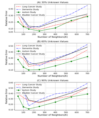Figure 1. Comparison of relative errors for different values of k for KNN method.

For the aim of finding the best k for KNN method, we varied the value of k from the list 50, 100, 150, 250, 400, 550, 700 and calculated the relative error in cases where 30%, 60% and 90% of the values are unknown. As Figure 1 shows, when the value is around 150-250, the relative error is the least so we selected 200 as the number of neighbors. The results of the comparison between KNN algorithm and PCC- CMC method are summarized in table 1. KNN method is extremely slow when the size of the dataset is large.

Table 1. Comparison of relative error averages for 4 datasets of KNN method and PCC-CMC

	KNN (k = 200)	PCC-CMC
30% Unknowns	0.103	0.047
60% Unknowns	0.169	0.069
90% Unknowns	0.225	0.102

We compared the performance of nuclear norm minimization to PCC, ED and CS based correlation approach on 4 NCBI-GEO datasets (Dementia, Autism, Lung cancer and Bladder cancer) and results are displayed in figure 2. The horizontal axis of all graphs (A – H) represents the ratio of the missing entries. The vertical axis of graphs A, C, E and G represents the relative error (Eq. 43) and the vertical axis in graphs B, D, F and H shows mean squared error (Eq. 44). The performance of PCC-CMC approach is shown by the dotted red line while the black, the dotted blue and the green lines depict the performances of the ED-CMC, CS-CMC and nuclear norm minimization approaches respectively. As the figure 2. Shows, for all four datasets, the PCC-CMC approach consistently beats the nuclear norm minimization approach. The nuclear norm minimization (green line) represents an increasingly growing error but the error of the PCC-CMC approach (red line) shows a decreasing acceleration. The CS-CMC (blue line) also represents improvements when compared to nuclear norm minimization but the ED-CMC approach does not show any improvements. The relative error and mean squared error of PCC-CMC grew very much slower than that of the nuclear norm minimization approach in cases of an increase in the ratio of missing entries. We can explain the different results of PCC-CMC and CS-CMC by this hypothesis that PCC might be better in catching the genes correlation compared to CS.

Based on our results, The PCC-CMC approach has higher accuracy compared to other approaches. In the case of 90% missing values for relative error, in the best case, PCC-CMC outperforms CS-CMC, ED-CMC, and Nuclear norm minimization by a factor of 1.4, 2 and 2.2 respectively. In the worst case PCC-CMC outperforms CS-CMC, ED-CMC, and Nuclear norm minimization by a factor of 1.2, 1.6 and 1.7 respectively. When looking at MSE, PCC-CMC outperforms the other three approaches by as much as a factor of 1.7, 2.3 and 2.4 respectively (for the same order as previously) and in the worst case we get an improvement factor of 1.1, 1.3 and 1.4 respectively.

We then compared the performance of the featured ADMM approach to SVT, ELAM, ILAM and PCC-CMC approach for our 4 datasets and the results are presented in figure 3. The horizontal axis in all graphs (A – H) represents the ratio of the missing entries. The vertical axis in graphs A, C, E and G shows the relative error and the vertical axis in graphs B, D, F and H shows mean squared error. The performance of the featured ADMM approach is shown by the dotted red line while the black, the dotted blue, the green and the gray lines represent the performances of the SVT, ELAM, ILAM and PCC-CMC approaches respectively. As Figure 3. Shows, for all four datasets, the ADMM approach beats the other four approaches. The black,

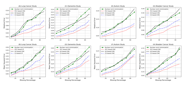Figure 2. Comparison of the performance of 4 different methods on NCBI-GEO dataset

Figure 3. Comparison of 5 different approaches on 4 NCBI-GEO datasets.

blue and green lines show increasingly growing errors but the errors of the red line show a decreasing acceleration. The mean squared error of the ADMM approach grows much slower than that of the other four in cases of an increase in the ratio of missing entries.

Based on our results, The ADMM approach has higher accuracy especially in the cases where the matrix has more missing values. In the case of 90% missing values for relative error, in the best case, ADMM outperforms PCC-CMC, ILAM, ELAM, and SVT by a factor of 1.85, 3, 3.3, and 4 respectively. In the worst case ADMM outperforms PCC-CMC, ILAM, ELAM, and SVT by a factor of 1.4, 1.3, 1.7 and 2 respectively. When looking at MSE, ADMM outperforms the other four approaches by as much as a factor of 2.2, 2.3, 3 and 4.8 respectively (for the same order as previously) and in the worst case we get an improvement factor of 1.6, 1.6, 2.3 and 3.4 respectively.

6. Conclusion

In this paper we employed three similarity metrics (Pearson Correlation Coefficient, Euclidean distance and Cosine Similarity) and Robust Principal Component Analysis (RPCA) on gene expression datasets. In section 2, we described the correlation based MC approach, the RPCA approach and also we briefly explained the Alternating Direction Method of Multipliers (ADMM) algorithm. We used 4 different gene expression datasets from NCBI and in the first step, we randomly removed a fraction of the entries (from 10% – 90%). So for each dataset we had 9 incomplete matrices that we aim to recover and predict the missing values using one the aforementioned approaches. When we measured the accuracy of the three correlation based approaches, K-nearest neighbors and a recent nuclear-norm minimization based approach, we found out the PCC-CMC approach outperforms the other methods.

In another experiment we evaluate the performance of ADMM approach. To do this, we described three well known algorithms that can be used when recovering low rank matrices and we compared the performances of them. We found that ADMM approach outperforms the other approaches.

 This paper can provide an inspiration for developing new approaches especially in gene expression studies and also has implications to recommender systems. There is a high demand for new efficient and fast methods to reduce the huge amount of time and resources that is often needed for gene expression studies.  Using such computational methods can help biologists find missing values in partially known gene expression datasets and also can help identify promising directions for studies based on partial measurements in gene expression experiments.

1.  N. Fraidouni and G. Zaruba, “A correlation based matrix completion approach to gene expression prediction,” in 7th International Conference on Computational Advances in Bio and Medical Sciences (ICCABS), Orlando, FL, 2017.
2.  N. Fraidouni and G. Zaruba, “A Robust Principal Component Analysis via Alternating Direction Method of Multipliers to Gene-Expression Prediction,” in Proceedings of the 2017 International Conference on Computational Science and Computational Inteligence (CSCI), Las Vegas, NV, 2017.
3.  R. Hammamieh, N. Chakraborty, A. Gautam and S. Muhie, “Whole-genome DNA methylation status associated with clinical PTSD measures of OIF/OEF veterans,” Transl Psychiatry, PMID: 28696412, 2017.
4.  Y. Bromberg, “Chapter 15: Disease gene prioritization,” PLoS Computational Biology, 2013.
5.  A. Wong, W. H. Au and K. Chen, “Discovering high-order patterns of gene expression levels,” Journal of Computational Biology, pp. 625-637, 2008.
6.  S. Welsh and S. Kay, “Reporter gene expression for monitoring gene transfer,” Current Opinions in Biotechnology, pp. 617-622, 1997.
7.  A. W. Liew, N. Law and H. Yan, “Missing value imputation for gene expression data: computational techniques to recover missing data from available information,” Briefings in Bioinformatics, vol. 12, no. 5, pp. 495-513, 2011.
8.  V. Gligorijevic and N. Przulj, “Computational Methods for Integration of Biological Data,” Springer International Publishing, pp. 137-178, 2016.
9.  X. Feng and X. He, “Inference on low rank data matrices with applications to microarray data,” The Annuals of Applied Statistics, pp. 217-243, 2010.
10.  F. O. Isinkaye, Y. O. Folajimi and B. A. Ojokoh, “Recommendation systems: Principles, methods and evaluation,” Egyptian Informatics Journal, vol. 16, no. 3, pp. 261-273, 2015.
11.  A. M. Acilar and A. Arslan, “A collaborative filtering method based on Artificial Immune Network,” Expert Systems with Applications, vol. 36, no. 4, pp. 8324-8332, 2009.
12.  L. S. Chen, F. H. Hsu, M. C. Chen and Y. C. Hsu, “Developing recommender systems with the consideration of product profitability for sellers,” International Journal of Geographical Information Science, vol. 187, no. 4, pp. 1032-1048, 2008.
13.  M. Jalali, N. Mustafa, M. Sulaiman and A. Mamay, “WEBPUM: a web-based recommendation system to predict user future movement,” Expert Systems with Applications, vol. 37, no. 9, pp. 6201-6212, 2010.
14.  M. Ekstrand, J. T. Reidl and J. Konstan, “Collaborative Filtering Recommender Systems,” Foundations and Trends in Human–Computer Interaction, vol. 4, pp. 81-173, 2011.
15.  Y. El Madani El Alami, E. H. Nfaoui and O. El Beqqali, “Improving Neighborhood-Based Collaborative Filtering by A Heuristic Approach and An Adjusted Similarity Measure,” in Proceedings of the International Conference on Big Data, Cloud and Applications, Tetuan, Morocco, 2015.
16.  F. Alqadah, C. Reddy and J. Hu, “Biclustering neighborhood-based collaborative filtering method for top-n recommender systems,” Springer-Verlag London, 2014.
17.  X. Zhou, C. Yang, H. Zhao and W. Yu, “Low-Rank Modeling and Its Applications in Image Analysis,” ACM Computing Surveys, vol. 47, no. 2, 2014.
18.  J. Gillard and K. Usevich, “Structured low-rank matrix completion for forecasting in time series analysis,” Elsevier, 2018.
19.  E. C. Lai, P. Tomancak, R. W. Williams and G. M. Rubin, “Computational identification of Drosophila MicroRNA genes,” Genome Biology, vol. 4, 2003.
20.  E. Candes and B. Recht, “Exact matrix completion via convex optimization,” Applied and Computational Mathematics, 2008.
21.  J. Wright, Y. Peng and Y. Ma, “Robust principal component analysis: exact recovery of corrupted low rank matrices by convex optimization,” in NIPS, 2009.
22.  J. F. Cai, E. J. Candes and Z. Shen, “A singular value thresholding algorithm for matrix completion,” SIAM Journal of Optimization, vol. 20, no. 4, pp. 1956-1982, 2010.
23.  I. Daubechies, M. Defrise and C. De Mol, “An iterative thresholding algorithm for linear inverse problems with a sparsity constraint,” Communications on Pure and Applied Mathematics, 2008.
24.  S. Taneja, C. Gupta, K. Goyal and D. Gureja, “An enhanced K-nearest neighbor algorithm using information gain and clustering,” in Fourth International Conference on Advanced Computing & Communication Technologies, 2014.
25.  A. Kapur, K. Marwah and G. Alterovitz, “Gene expression prediction using low-rank matrix completion,” BMC Bioinformatics, pp. 1634-1654, 2016.
26.  Z. Lin, M. Chen and Y. Ma, “The augmented lagrange multiplier method for exact recovery of corrupted low-rank matrices,” Mathematical Programming, 2010.
27.  Z. Lin, M. Chen and Y. Ma, “Linearized Alternating Direction Method with Adaptive Penalty for Low Rank Representation,” in Conference on Neural Information Processing Systems (NIPS), 2011.
28.  M. T. Landi, T. Dracheva, M. Rotunno and J. D. Figueroa, “Gene expression signature of cigarette smoking and its role in lung adenocarcinoma development and survival,” PLoS One, PMID: 18297132, 2008.
29.  A. S. Chen-Plotkin, F. Geser, J. B. Plotkin and C. M. Clark, “Variations in the progranulin gene affect global gene expression in frontotemporal lobar degeneration,” Human Molecular Genetics, vol. 17, no. 10, p. PMID: 18223198, 2008, PMID: 18223198.
30.  M. D. Alter, R. Kharkar, K. E. Ramsey and D. W. Craig, “Autism and increased paternal age related changes in global levels of gene expression regulation,” Plos One, vol. 6, no. 2, p. PMID: 21379579, 2011.
31.  M. Riester, J. M. Taylor, A. Feifer and T. Koppie, “Combination of a novel gene expression signature with a clinical nomogram improves the prediction of survival in high-risk bladder cancer,” Clinical Cancer Research, PMID: 22228636, 2012.

(Click Here)

(Click Here)