1. Introduction

Voice problems are a common reason for referrals by primary practices to ear, nose and throat (ENT) departments and voice clinics in hospitals. Such problems may result from voice-strain due to speaking or singing excessively or too loudly, vocal cord inflammation, side-effects of inhaled steroids as used to treat asthma, infections, trauma, neoplasm, neurological disease and many other causes. This paper is an extension of work on voice quality assessment originally presented in the 10th CISP-BMEI, conference in Shanghai [1].  Speech and language therapists (SLTs) are commonly required to assess the nature of voice quality impairment in patients, by audio-perception.  This requires the SLT, trained as a voice quality expert, to listen to and assess the patient’s voice while it reproduces, or tries to reproduce, certain standardized vocal maneuvers.  In Europe, voice quality assessments are often made according to the perception of five properties of the voice as proposed by Hirano [2]. The five properties are referred to by the acronym ‘GRBAS’ which stands for ‘grade’, ‘roughness’, ‘breathiness’, ‘asthenia’ and ‘strain’. Each GRBAS property is rated, or scored by assigning an integer 0, 1, 2 or 3.  A score of 0 signifies no perceived loss of quality in that property, 1 signifies mild loss of quality, 2 signifies moderate loss and 3 signifies severe loss.   The scoring may be considered categorical or ordinal.  With categorical scoring the integers 0, 1, 2 and 3 are considered as labels.  With ordinal scoring, the integers are considered as being numerical with magnitudes indicating the severity of the perceived quality loss.

Grade (G) quantifies the overall perception of voice quality which will be adversely affected by any abnormality. Roughness (R) measures the perceived effect of uncontrolled irregular variations in the fundamental-frequency and amplitude of vowel segments which should be strongly periodic. Breathiness (B) quantifies the level of sound that arises from turbulent air-flow passing through vocal cords when they are not completely closed.  Asthenia (A) measures the perception of weakness or lack of energy in the voice.  Strain (S) gives a measure of undue effort needed to produce speech when the speaker is unable to employ the vocal cords normally because of some impairment.

Voice quality evaluation by audio-perception is time-consuming and expensive in its reliance on highly trained SLTs [3].  Also, inter-rater inconsistencies must be anticipated, and have been observed [4] in the audio-perceptual scoring of groups of patients, or their recorded voices, by different clinicians.  Intra-rater inconsistencies have also been observed when the same clinician re-assesses the same voice recordings on a subsequent occasion.  A lack of consistency in GRBAS assessments can adversely affect the appropriateness of treatment offered to patients, and the monitoring of its effect. A computerized approach to GRBAS assessment could eliminate these inconsistencies.

According to Webb et al. [5], GRBAS is simpler and more reliable than many other perceptual voice evaluation scales, such as Vocal Profile Analysis (VPA) [6] and the ‘Buffalo Voice Profile’ (BVP) [7], scheme.  The ‘Consensus Auditory-Perceptual Evaluation of Voice’ (CAPE-V) approach, as widely used in North America [8], allows perceptual assessments of overall severity, roughness, breathiness, strain, pitch and loudness to be expressed as percentage scores.  It is argued [8] that, compared with GRBAS, the CAPE-V scale better measures the quality of the voice and other aphonic characteristics.  Also, CAPE-V assessments are made on a more refined scale.  However, GRBAS is widely adopted [9] by practicing UK voice clinicians as a basic standard.

No definitive solutions yet exist for performing GRBAS assessments by computer.  Some approaches succeeded in establishing reasonable correlation between computerized measurements of acoustic voice features and GRBAS scores, but have not progressed to prototype systems [12]. Viable systems have been proposed, for example [13], but problems of training the required machine learning algorithms remain to be solved.  The ‘Multi-Dimensional Voice Program’ (MDVP) and ‘Analysis of Dysphonia in Speech and Voice’ (ADSV) are commercial software packages [10] providing a wide range of facilities for acoustic feature analysis.  Additionally, ADSV gives an overall assessment of voice dysphonia referred to as the Cepstral/spectral Index of Dysphonia (CSID) [11].  This is calculated from a multiple regression based on the correlation of results from ADSV analyses with CAPE-V perceptual analyses by trained scorers.  The CAPE-V overall measure of dysphonia is closely related to the ‘Grade’ component of GRBAS, therefore the CSID approach offers a methodology and partial solution to the GRBAS prediction problem.  However the commercial nature of the CSID software makes it difficult to study and build on this methodology.  Therefore, this paper considers how the results of a GRBAS scoring exercise may be used to produce a set of reference scores for training machine learning algorithms for computerized GRBAS assessment.

For the purposes of this research, a scoring exercise was carried out with the participation of five expert SLT raters, all of whom were trained and experienced in GRBAS scoring and had been working in university teaching hospitals for more than five years. A database of voice recordings from 64 patients was accumulated over a period of about three months by randomly sampling the attendance at a typical voice clinic. This database was augmented by recordings obtained from 38 other volunteers.

The recordings were made in a quiet studio at the Manchester Royal Infirmary (MRI) Hospital.  Ethical approval was given by the National Ethics Research committee (09/H1010/65). The KayPentax 4500 CSL ® system and a Shure SM48 ® microphone were used to record the voices with a microphone set at 45 degrees at a distance of 4 cm.  The recordings were of sustained vowel sounds and segments of connected speech.

To obtain the required GRBAS scores for each of the subjects (patients and other volunteers), the GRBAS properties of the recordings were assessed independently by the five expert SLT raters with the aid of a ‘GRBAS Presentation and Scoring Package (GPSP)’ [14].  This application plays out the recorded sound and prompts the rater to enter GRBAS scores.  Raters used Sennheiser HD205 ® head-phones to listen to the recorded voice samples. The voice samples are presented in randomized order with a percentage (about 20 %) of randomly selected recordings repeated without warning, as a means of allowing the self-consistency of each rater to be estimated.

Different statistical methods were then employed to measure the intra-rater consistency (self-consistency) and inter-rater consistency of the scoring. Some details of these methods are presented in the next section.  The derivation of ‘reference’ GRBAS scores from the audio-perceptual rater scores is then considered for the purpose of training ML algorithms for computerized GRBAS scoring.  The derivation takes into account the inter-rater and intra-rater consistencies of each rater,

Voice quality assessment may be computerized using digital signal processing (DSP) techniques which analyze recorded segments of voice to quantify universally recognized acoustic features such as fundamental frequency, shimmer, jitter and harmonic-to-noise ratio [14].  Such acoustic features are not obviously related to the GRBAS measurements that are widely recognized and understood by clinicians.  We therefore investigated the use of machine learning (ML) for mapping these feature measurements to the more familiar GRBAS assessments.  Our approach was to derive ‘reference scores’ for a database of voice recordings from the scores given by expert SLT raters.  The reference scores are then used to train a machine-learning algorithm to predict GRBAS scores from the acoustic feature measurements resulting from the DSP analysis. The effectiveness of these techniques for computerised GRBAS scoring is investigated in Section 13 of this paper.

2. Measurement of Consistency

The properties of a number of well-known statistical methods for measuring rater consistency were considered for this research.   The degree of consistency between two raters when they numerically appraise the same phenomena may be measured by a form of correlation.  Perhaps the best known form of correlation is Pearson Correlation [15].  However, this measure takes into account only variations about the individual mean score for each rater [16].  Therefore a rater with consistently larger scores than those of another rater can appear perfectly correlated and therefore consistent with that other rater.  Pearson correlation has been termed a measure of ‘reliability’ [17] rather than consistency. It is applicable only to ordinal appraisals, and is generally inappropriate for measuring consistency between or among raters [9] where consistency implies agreement.  The notion of consistency between two raters can be extended to self-consistency between repeated appraisals of the same phenomena by the same rater (test-retest consistency), and to multi-rater consistency among more than two raters.

An alternative form of correlation is given by the ‘intra-class correlation’ coefficient (ICC) [18] and this may be used successfully as a measure of consistency for rater-pairs.  It is also suitable for intra-rater (test-retest) and multi-rater consistency.  The scoring must be ordinal.  ICC is based on the differences that exist between the scores of each rater and a ‘pooled’ arithmetic mean score that is computed over all the scores given by all the raters.  Therefore ICC eliminates the disadvantage of Pearson Correlation that it takes into account only variations about the individual mean score for each rater.

The ‘proportion of agreement’ (P_o), for two raters, is a simple measure of their consistency.  It is derived by counting the number of times that the scores agree and dividing by the number, N, of subjects.   P_o will always be a number between 0 (signifying no agreement at all) and 1 (for complete agreement).  It is primarily for categorical scoring but may also be applied to ordinal scoring where the numerical scores are considered as labels.  For ordinal scoring, P_o does not reflect the magnitudes of any differences, and in both cases, P_o is biased by the possibility of agreement by chance.  The expectation of P_o will not be zero for purely random scores because some of the scores will inevitably turn out to be equal by chance. With Q different categories or scores evenly distributed over the Q possibilities, the probability of scores being equal by chance would be 1/Q.  Therefore, the expectation of P_o would be 1/Q rather than zero for purely random scoring.  With Q = 4, this expectation would be a bias of 0.25 in the value of P_o.  The bias could be even greater with an uneven spread of scores by either rater.  The bias may give a false impression of some consistency when there is none, as could occur when the scores are randomly generated without reference to the subjects at all.

The Cohen Kappa is a well known consistency measure originally defined [19] for categorical scoring by two raters.  It was later generalised to the weighted Cohen Kappa [20] which is applicable to ordinal (numerical) scoring with the magnitudes of any disagreements between scores taken into account.  The Fleiss Kappa [21] is a slightly different measure of consistency for categorical scoring that may be applied to two or more raters.  The significance of Kappa and ICC measurements is often summarised by descriptions [22, 23] that are reproduced in Tables 1 and 2.  A corresponding table for the Pearson correlation coefficient may be found in the literature [24].

Table 1: Significance of Kappa Values

Kappa	Consistency
1.0	Perfect
0.8 – 1.0	Almost perfect
0.6 – 0.8	Substantial
0.4 – 0.6	Moderate
0.2 – 0.4	Fair
0 – 0.2	Slight
< 0	Less than chance

Table 2: Significance of ICC Values

ICC	Consistency
0.75 – 1.0	Excellent
0.4 – 0.75	Fair
< 0.4	Poor

3. The Cohen Kappa

The original Cohen Kappa [19] for two raters, A and B say, was defined as follows:

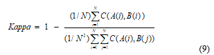
where P_o is the proportion of agreement, as defined above, and P_e is an estimate of the probability of agreement by chance when scores by two raters are random (unrelated to the patients) but distributed across the range of possible scores identically to the actual scores of raters A and B.  The estimate P_e is computed as the proportion of subject pairs (i ,j) for which the score given by rater A to subject i is equal to the score given by rater B to subject j.  This is an estimate of the probability that a randomly chosen ordered pair of subjects (i, j) will have equal scores.

This measure of consistency [19] is primarily for categorical scoring, though it can be applied to ordinal scores considered as labels.  In this case, any difference between two scores will be considered equally significant, regardless of its numerical value.  Therefore, it will only be of interest whether the scores, or classifications, are the same or different.

The weighted Cohen Kappa [20] measures the consistency of ordinal scoring where numerical differences between scores are considered important.  It calculates a ‘cost’ for each actual disagreement and also for each expected ‘by chance’ disagreement.  The cost is weighted according to the magnitude of the difference between the unequal scores. To achieve this, equation (1) is re-expressed by equation (2):

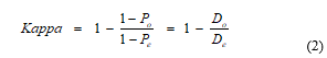where D_o = 1 – P_o is the proportion of actual scores that are not equal and is considered to be the accumulated cost of the disagreements.  The quantity D_e = 1 – P_e is now considered to be the accumulated cost of disagreements expected to occur ‘by chance’ with random scoring distributed identically to the actual scores.  Weighting is introduced by expressing D_o and D_e in the form of equations (3) and (4):

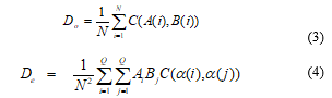In equations (3) and (4), C(a,b) is the cost of any difference between scores (or categories) a and b.  In equation (4), A_i denotes the number of subjects that rater A scores as a(i) and B_j denotes the number of subjects that rater B scores as a(j).  Q is the number of possible scores or scoring categories and these are denoted by a(1), a(2)… a(Q).  If the cost-function C is defined by equation (5):

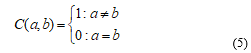the weighted Cohen Kappa [20] becomes identical to the original Cohen Kappa [19] also referred to as the unweighted Cohen Kappa (UwCK).  If C is defined by equation (6),

we obtain the ‘linearly weighted Cohen Kappa’ (LwCK), and defining C by equation (7) produces the ‘quadratically weighted Cohen Kappa’(QwCK).

There are other cost-functions with interesting properties, but the three mentioned above are of special interest.  For GRBAS scoring, there are Q = 4 possible scores which are a(1)=0, a(2)=1, a(3)=2 and a(4)=3.

Equation (4) may be re-expressed as equation (8):

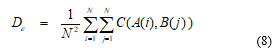Therefore, from equations (2), (3) and (8), we obtain equation (9) which is a general formula for all 2-rater (pair-wise) forms of Cohen Kappa:

The original and weighted Cohen Kappa [19, 20] are applicable when there are two individual raters, A and B say, who both score all the N subjects. The raters are ‘fixed’ in the sense that rater A is always the same clinician who sees all the subjects; and similarly for rater B.  Therefore the individualities and prejudices of each rater can be taken into account when computing P_e, the probability of agreement by chance.  For example, if one rater tends to give scores that are consistently higher than those of the other rater, this bias will be reflected in the value of Cohen Kappa obtained.

4. Other Versions of Kappa

The Fleiss Kappa [21] measures the consistency of two or more categorical raters, and can therefore be a ‘multi-rater’ consistency measure.  Further, the raters are not assumed to be ‘fixed’ since each subject may be scored by a different pair or set of raters.   Therefore, it is no longer appropriate to take into account the different scoring preferences of each rater.  If the Fleiss Kappa is used for a pair of fixed raters as for the Cohen Kappas, slightly different measurements of consistency will be obtained.

Assuming that there are n raters and Q scoring categories, Fleiss [21] calculates the proportion p_j of the N subjects that are assigned by raters to category j, as follows:

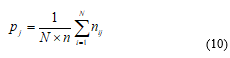for j = 1, 2, …, Q, where n_ij is the number of raters who score subject i as being in category j.  The proportion, P_i, of rater-pairs who agree in their scoring of subject i is given by:

where L is the number of different rater-pairs that are possible, i.e. L = n(n-1)/2.  The proportion of rater-pairs that agree in their assignments, taking into account all raters and all subjects, is now:

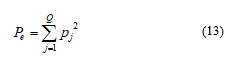
Fleiss [21] then estimates the probability of agreement ‘by chance’ as:

Substituting from equations (12) and (13) into the Kappa equation (1) gives the Fleiss Kappa [21] which may be evaluated for two or more raters not assumed to be ‘fixed’ raters.  The resulting equation does not generalise the original Cohen Kappa because equation (13) does not take any account of how the scores by each individual rater are distributed.  P_e is now dependent only on the overall distribution of scores taking all raters together.   Agreement by chance is therefore redefined for the Fleiss Kappa.

The original Cohen Kappa may be truly generalised [27] to measure the multi-rater consistency of categorical scoring by a group of n ‘fixed’ raters, where n ³ 2.  Light [28] and Hubert [29] published different versions for categorical scoring, and Conger [30] extended the version by Light [28] to more than three raters.  The generalisation by Hubert [29] redefines D_o and D_e to include all possible rater-pairs as in equation (14):

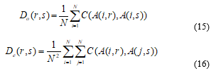
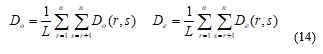where the expression for D_o(r,s) generalizes equation (3) and the expression for D_e(r,s) generalizes equation (8) to become the cost of actual disagreement and the expected cost of by chance disagreement between raters r and s.  Denoting by A(i, r) the score given by rater r to subject i, we obtain equations (15) and (16):

where equation (5) defines the cost-function C.  Substituting for D_o and D_e from equation (14) into equation (2), with D_o(r,s) and D_e(r,s) defined by equations (15) and (16) gives a formula for the multi-rater Cohen Kappa that is functionally equivalent to that published by Hubert [29].  With C defined by equation (5) it remains unweighted.

The generalization by Light [28] is different from the Hubert version when n > 2.  It is given by equation (17):

Although both generalizations were defined for categorical scoring, they may now be further generalised to weighted ordinal scoring simply by redefining the cost-function C, for example by equation (6) for linear weighting or equation (7) for quadratic weighting.  With n = 2, both generalisations are identical to the original [19] or weighted [20] Cohen Kappa.

5. Weighted Fleiss Kappa

As explained in [31], the original Fleiss Kappa [21] is given by equation (18) when the cost-function C is as in equation (5).

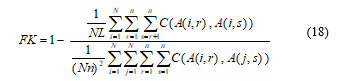The Fleiss Kappa may be generalized to a weighted version for ordinal scoring by redefining cost-function C as for the multi-rater Cohen Kappa.  In all cases, the unweighted or weighted Fleiss Kappa is applicable to measuring the consistency of any number of raters including two.

6. Intra-Class Correlation Coefficient (ICC)

In its original form [25], ICC is defined for n raters as follows:

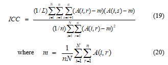Other versions of ICC have also been proposed [26].  It is known [26] that, for two raters, ICC will be close to quadratically weighted Cohen Kappa (QwCK) when the individual mean score for each rater is approximately the same.  This property is observed [31] also for multi-rater versions of ICC and QwCK.  More interestingly, it has been shown [31] that ICC is always exactly equal to quadratically weighted Fleiss Kappa (QwFK) regardless of the number of raters and their individual mean scores.

7. Intra-rater Consistency

For the GRBAS rating exercise referred to in Section 1, intra-rater (test-retest) scoring differences were generally small due to the experience and high expertise of the SLT raters.  There were some differences of 1, very occasional differences of 2, and no greater differences.  The test-retest consistency for the five GRBAS components was measured for all five raters, by unweighted, linearly weighted and quadratically weighted Cohen Kappa (UwCK, LwCK and QwCK) and ICC.  By averaging UwCK, LwCK and pair-wise ICC measurements over the five GRBAS components we obtained Table 3 which gives three overall measurements of the test-retest consistency of each rater.  QwCK gave a close approximation to ICC, and is not shown in the table.  QwFK, also not shown, was indistinguishable from ICC.  For all forms of Kappa, the P_o and P_e terms were averaged separately.  Similarly, the ICC numerators and denominators were averaged separately.

With UwCK, any difference in scores incurs the same cost regardless of its magnitude.  Small differences cost the same as large differences.  This makes UwCK pessimistic for highly consistent raters where most test-retest discrepancies are small.   Therefore, the averaged UwCK consistency measurements in Table 3 are pessimistic for our rating exercise.

With QwCK, the largest differences in scores incur very high cost due to the quadratic weighting.  With ICC, the costs are similar.  These high costs are important even when there are few or no large scoring differences because they strongly affect the costs of differences expected to incur ‘by chance’.  These high ‘by chance’ costs make both QwCK and ICC optimistic, when compared with LwCK, for highly consistent rating with a fairly even distribution of scores.  We therefore concluded that LwCK gives the most indicative measure of test-retest consistency for the rating exercise referred to in this paper.  A different set of scores may have led to a different conclusion.   In Table 3, it may be seen that the self-consistency of raters 1 to 4, as measured by LwCK, was considered ‘substantial’ according to Table 2.  The self-consistency of rater 5 was considered ‘moderate’.  Conclusions can therefore be drawn about the self-consistency of each rater and how this may be expected to vary from rater to rater.

Table 3: Intra-Rater Consistency Averaged over all GRBAS Components

Rater	UwCK	LwCK	ICC	Consistncy (LwCK)	Consistncy (ICC)
1	0.72	0.77	0.84	Substantial	Excellent
2	0.65	0.76	0.85	Substantial	Excellent
3	0.53	0.64	0.75	Substantial	Excellent
4	0.68	0.73	0.77	Substantial	Excellent
5	0.44	0.60	0.74	Moderate	Fair

Table 4: Intra-rater Consistency Averaged over all 5 raters

Comp- onent	UwCK	LwCK	ICC	Consistncy (LwCK)	Consistncy (ICC)
G	0.64	0.77	0.87	Substantial	Excellent
R	0.57	0.67	0.76	Substantial	Excellent
B	0.55	0.66	0.76	Substantial	Excellent
A	0.68	0.73	0.80	Substantial	Excellent
S	0.59	0.68	0.76	Substantial	Excellent

Table 4 shows UwCK, LwCK and ICC intra-rater consistency measurements for G, R, B, A, and S, averaged over all five raters.  According to all the measurements, it appears that test-retest consistency with R, B and S is more difficult to achieve than with G and A.

8. Inter-rater Consistency

Measurements of inter-rater consistency between pairs of raters for any GRBAS component may be obtained using the same forms of Kappa and ICC as were used for intra-rater consistency.  Our rating exercise had a group of five raters, therefore ten possible pairs.  This means that there are ten pair-wise measurements of inter-rater consistency for each GRBAS component.  To reduce the number of measurements, it is convenient to define an ‘individualised’ inter-rater measurement for each rater.  For each GRBAS component, this individualized measurement quantifies the consistency of the rater with the other raters in the group.  It is computed for each rater by averaging all the pair-wise inter-rater assessments which involve that rater.  Thus an individualized measure of inter-rater consistency is obtained for G, R, B, A and S for each rater.  With five raters, the 25 measurements can be reduced to five by averaging the individualized G, R, B, A and S measurements to obtain a single average measure for each rater.

The UwCK, LwCK and ICC individualized inter-rater measurements, averaged over all GRBAS components, are shown in Table 5 for raters 1 to 5.  For all raters, the average consistency is ‘moderate’ according to LwCK and ‘fair’ according to ICC.  Raters 1, 4 and 5 have almost the same inter-rater consistency, rater 2 has slightly lower consistency and rater 2 is the least consistent when compared with the other raters.

Table 5: Individualized Inter-rater Consistency averaged over all GRBAS Components

Rater	UwCK	LwCK	ICC	Consistncy (LwCK)	Consistncy (ICC)
1	0.47	0.59	0.70	Moderate	Fair
2	0.40	0.52	0.60	Moderate	Fair
3	0.45	0.57	0.67	Moderate	Fair
4	0.48	0.60	0.71	Moderate	Fair
5	0.47	0.59	0.70	Moderate	Fair

9. Multi-rater Consistency

The multi-rater consistency according to the unweighted Fleiss Kappa (FK), the generalised Cohen Kappa (with linear weighting) and ICC, computed for the group of five raters, are shown in Table 6 for each GRBAS component. The values of UwCK were indistinguishable from FK  to the precision shown in the table.  Similarly for the values of QwCK and ICC.  Quadratically weighted FK, also not shown, would be exactly equal to ICC.

Table 6: Multi-rater Consistency by Fleiss Kappa, Cohen Kappa and ICC

	FK	LwCK	ICC	Consistncy (LwCK)	Consistncy (ICC)
G	0.56	0.71	0.83	Substantial	Excellent
R	0.44	0.57	0.68	Moderate	Fair
B	0.43	0.58	0.71	Moderate	Fair
A	0.38	0.46	0.55	Moderate	Fair
S	0.44	0.54	0.65	Moderate	Fair

In contrast to Table 5 which allows us to compare the overall consistency of raters, Table 6 allows us to compare the difficulty of achieving group consistency for each GRBAS component. It is clear that some GRBAS components are more difficult to score consistently than others.  According to ICC, group consistency is ‘excellent’ for Grade and ‘fair’ for R, B, A and S.  LwCK gives ‘substantial’ for Grade and ‘fair’ for the others. The FK and UwCK measurements are more pessimistic due to their assumption that the scoring is categorical.  According to all measurements of multi-rater consistency, the consistency is highest for highest, followed by Breathiness, Roughness, Strain and Asthenia.

It should be mentioned that the classifications given by Tables 1 and 2 serve only as a rough guide to interpreting the values of Kappa and ICC obtained.  However, they are widely used despite the fact that it seems inappropriate to use Table 2 for quadratically weighted Kappa in view of its closeness to ICC.  In particular, the category ‘Fair’ in Tables 2 and 3 refers to quite different ranges which may be misleading if Table 2 were used for QwCK.  Therefore, it is appropriate to refer to Table 3 for both ICC and quadratically weighted Kappa.

10. Reference GRBAS Scores

The feasibility of performing automatic GRBAS scoring by computer was investigated by training machine learning (ML) algorithms for mapping acoustic feature measurements to the familiar GRBAS scale.  For the training, a set of accurate and reliable GRBAS scores was required for each of the N subjects in our database. We refer to these as ‘reference’ GRBAS scores.  A technique for deriving these reference scores from the scores of a group of audio-perceptual raters, such as that described in Section 1, was therefore devised.  The measurements of inter-rater and intra-rater consistency, obtained as described above, is taken into account as a means of optimising the accuracy and reliability of the reference scores.

Given the ‘Grade’ scores A(i, r) for subject i, with rater-index r in the range 1 to 5, we first computed weighted average pair-wise scores G_rs(i) by equation (21), for all possible rater-pairs (r,s).  The weighting is by the LwCK intra-rater consistency measurements in Table 3 referred to now as w₁, w₂, w₃, w₄, w₅ for raters 1 to 5 respectively.

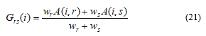The ‘Grade’ reference score for subject i is then obtained as a weighted average of the G_rs(i) values over all possible rater-pairs,  i.e.:

where L = n(n-1)/2 with n=5.  The weights w(r,s) are the pair-wise inter-rater LwCK measurements for Grade.  This procedure is performed for all subjects for Grade, and then repeated for the other GRBAS dimensions.  The weighting de-emphasises scores from less self-consistent raters in favour of more self-consistent ones.  It also de-emphasises the scores from raters who are less consistent with other raters.

11. Voice Quality Assessment by Computer

Considerable published research, including [12] and [13], has not yet established a definitive methodology for GRBAS assessment by computer.  An overall CAPE-V assessment of dysphonia, CSID [11], available commercially, is strongly related to ‘Grade’, but it does not independently assess the other GRBAS and CAPE-V components [8].  Computerised voice quality assessment may be carried out using digital signal processing (DSP) to analyse segments of voice to produce mathematical functions such as the autocorrelation function, fast Fourier Transform and cepstrum.  From such functions, acoustic features such as the aperiodicity index (API), fundamental frequency (F₀), harmonic-to-noise ratio (HNR), jitter, shimmer, cepstral peak prominence (CPP), low-to-high spectral ratio (LH) and others may be derived.  However, these features are not obviously related to GRBAS assessments of voice quality.

Perceived voice quality is strongly dependent on the short term periodicity of the vowels and the nature of the fluctuations in this periodicity.  To measure short-term periodicity, and how this varies over a spoken vowel, speech must be segmented into frames.  The degree of periodicity of each of these frames may expressed as an aperiodicity index (API) which is equal to 1 – p where p is the peak value of a suitable form of autocorrelation function.  An API of zero indicates exact periodicity and its value increases towards 1 with increasing aperiodicity.  The API is increased by additive noise due to ‘breathiness’, fundamental frequency or amplitude variation due to ‘roughness’ in the operation of the vocal cords, and other acoustic features.

A sustained vowel without obvious impairment will generally have strong short-term periodicity for the duration of the segment, though the fundamental frequency (F₀) and loudness may vary due to natural characteristics of the voice and controlled intonation.  By monitoring how the degree of short term periodicity changes over a passage of natural connected speech, vowels may be differentiated from consonants, thus allowing the acoustic feature measurements to concentrate on the vowels.

Jitter is rapid and uncontrolled variation of F₀ and shimmer is rapid and uncontrolled variation of amplitude.  Both these acoustic features can be indicative of roughness in GRBAS assessments.  They will affect grade also.  There are many ways of defining jitter and shimmer as provided by the Praat software package [32].  The HNR may be derived from the autocorrelation function and can be indicative of breathiness in GRBAS assessments since the ‘noise’ is often due to turbulent airflow.  Low-to-high spectral ratio (LH) measurements are made by calculating and comparing, in the frequency-domain, the energy below and above a certain cut-off frequency, such as 1.5 kHz or 4.0 kHz.   The required filtering may be achieved either by digital filters or an FFT. A high value of LH with cut-off frequency 1.5 kHz can be indicative of asthenia [36] and strain [37] due to imperfectly functioning vocal cords damping the spectral energy of formants above 1.5 kHz.  LH measurements with a cut-off frequency of 4.0 kHz are useful for detecting breathiness and voicing since the spectral energy of voiced speech (vowels) is mostly below 4.0 kHz.  CPP is widely used as an alternative to API and HNR as a means of assessing the degree of short term periodicity.

As in [34], well known DSP techniques were employed [14, 35] to recognise vowels and measure the acoustic features mentioned above, and several others.  Frame-to-frame variations in these features over time were also measured.  Published DSP algorithms and commercial and academic computer software are available for making these measurements from digitised voice recordings [32, 33].  Twenty acoustic features were identified by Jalalinajafabadi [14] as being relevant to GRBAS scores.  They were measured by a combination of DSP algorithms specially written in MATLAB and commercial software provided by MDVP and ADSV [10, 11].  For the MATLAB algorithms, the speech recordings were sampled at Fs = 44.1 kHz, and divided into sequences of 75% overlapping 23.22 ms frames of 1024 samples.  MDVP and ADSV use a slightly different sampling rate and framing.  Many of the features were strongly correlated and their usefulness was far from uniform.  Therefore, some experiments with feature selection were performed.  The usefulness of each possible sub-set of features for predicting each GRBAS component was estimated by a combination of correlation measurements, to reduce the dimensionality of the task, and then a form of direct search.  The use of Principle Component Analysis’ (PCA) would have reduced the computation, but this was not a critical factor.

Section 14 will evaluate the performance of MLR and KNNR (with and without feature selection) and perceptual analysis against the ‘reference GRBAS scores’.

12. Machine Learning Algorithms

We analysed the recordings of sustained vowels obtained from the N = 102 subjects mentioned in Section 1.  For each recording, acoustic feature measurements were obtained as explained in Section 11.  A total of m = 20 feature measurements were obtained as detailed in [14].   An N×m matrix X of feature measurements was defined for each of the five GRBAS components.  These matrices became the input to the machine learning (ML) algorithm along with the N´1 vector Y of reference GRBAS scores derived as explained in Section 10.  The ML algorithm was designed to learn to predict, as closely as possible, the reference GRBAS scores supplied for each subject. The prediction must be made from the information provided by the m acoustic feature measurements supplied for each voice segment.  Two simple ML approaches were compared [14, 35]: K-nearest neighbour regression (KNNR) and multiple linear regression (MLR).

With KNNR, the ML information consists of a matrix X and vector Y for each GRBAS component.  Supplying the ML algorithm with these arrays is all that is required of the training process.  K is an integer that defines the way the KNNR approach predicts a score for a new subject from measurements of its m acoustic features. The prediction is based on the known scores for K other subjects chosen according to the ‘distance’ of their measured acoustic features from those of the new subject.  The concept of distance can be defined in various ways such as the Euclidean distance which we adopted. The distance between the new subject and each of the N database subjects is calculated.  Then K subjects are selected as being those that are nearest to the new subject according to their feature measurements.  A simple form of KNNR takes the arithmetic mean of the scores of the K nearest neighbours as the result.  A preferred alternative form takes a weighted average where the reference scores are weighted according to the proximity of the reference subject to the new subject.

A choice of K must be made, and this may be different for each GRBAS component.  The optimal value of K will depend on the number, N, of subjects, the distribution of their scores and the number of acoustic features being taken into account.  K is often set equal the square root of N, though investigations can reveal more appropriate values.  In this work, Jalalinajafabadi [14] plotted the prediction error against K to obtain a suitable value of K for each GRBAS component.  This was done after selecting the most appropriate set of acoustic features for each GRBAS component. The values of K producing the lowest prediction errors were K=6 for grade, K=10 for roughness, K=5 for breathiness and K = 8 for strain and asthenia.

The Multiple Linear Regression (MLR) approach computes, for each GRBAS component, a vector b of K regression coefficients such that

where the error-vector e is minimized in mean square value over all possible choices of b of dimension K.  It may be shown [14] that the required vector b  is given by:

where X^# is the pseudo-inverse of the non-square matrix X.  For a subject whose m feature measurements x have been obtained, the equation:

produces a scoring estimate y.  This will be close to Y(i) for each subject i in our database, and may be expected to produce reasonable GRBAS scores for an unknown subject.

13. Testing and Evaluation

The application developed by Jalalinajafabadi [14] made m = 20 voice feature measurements per subject. Feature selection was applied to identify which subset of these m features gave the best result for each GRBAS dimension.  It was generally found that, compared with including all 20 feature measurements, better results were obtained with smaller subsets tailored to the GRBAS dimensions.  Several computational methods for feature selection were compared [14] in terms of their effectiveness and computational requirements.  The results presented here were obtained using a combination of correlation tables (between feature measurements and GRBAS components) and exhaustive search.  The best feature subsets for G, R, B, A and S are generally different, since different feature measurements highlight different aspects of the voice.  It was found beneficial to normalise the feature measurements to avoid large magnitudes dominating the prediction process, especially for KNNR.

To evaluate the KNNR and MLR algorithms for mapping acoustic feature measurements to GRBAS scores, 80 subjects were randomly selected for training purposes from the 102 available subjects.  The remaining 22 subjects were set aside to be used for testing the mapping algorithms once they had been trained.  Twenty ‘trials’ were performed by repeating the training and testing, each time with a different randomisation.  The same testing approach was used for both KNNR and MLR.  The trained mapping algorithm was used to predict GRBAS scores for the 22 testing subjects from the corresponding acoustic feature measurements.  The GRBAS scores thus obtained were compared with the known reference scores.  For each trial, a value of ‘root mean squared error’ (RMSE) was computed for each GRBAS component over the 22 testing subjects.  These RMSE values were then averaged over the 20 trials.  An RMSE of 100% would correspond to an RMS error of 1 in the GRBAS scoring where the averaging is over all 22 testing subjects and all 20 trials.

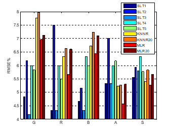Figure 1: RMSE% for SLT 1-5, KNNR & MLR with feature selection and using all available 20 features (KNNR20 & MLR20).

A comparison of the GRBAS scoring produced by the five SLTs and the KNNR and MLR algorithms is presented in Figure 1.  This graph summarises the results of experiments carried out by Jalalinajafabadi [14] with and without feature selection.  Measurements obtained without feature selection are labelled KNNR20 and MLR20 since all available 20 features are taken into account.  Comparing KNNR (with feature selection) and KNNR20, the feature selection has reduced the prediction error RMSE% by up to about 0.5%.  Comparing MLR and MLR20, the reduction due to feature selection is generally greater, i.e. about 1% for Roughness and up to 0.7% for the other components (apart from Grade).  With feature selection, the performances of the two machine learning techniques appear quite similar according to the RMSE measurements, though MLR is consistently better than KNNR.  For Asthenia and Strain, both KNNR and MLR with feature selection deliver a lower RMSE than was obtained for each of the SLT raters with reference to the corresponding reference-scores. For Grade, the KNNR and MLR values of RMSE (with feature selection) are both markedly higher than the corresponding values obtained for all the five SLT raters.  The worst RMS difference for Grade is about 7.5%.  The results for ‘Breathiness’ are close to those of the two worst performing SLT raters, and the MLR result for ‘Roughness’ lies between the two best and two worst performing SLT raters.  As reported by Jalalinajafabadi [14] and further explained in [1], the RMSE taken over all GRBAS components was found to be marginally lower for KNNR and MLR (both with feature selection) than for each of the five individual SLT raters.

14. Conclusions

Recordings of normal and impaired voices were obtained from randomly selected patients and some other volunteers.  These recordings were audio-perceptually assessed by five expert GRBAS raters to obtain a set of GRBAS scores for each recording.  Statistical methods for measuring the inter-rater and intra-rater consistency of the scoring were investigated and it was concluded that the linearly weighted Cohen Kappa (LwCK) was suitable for this purpose.  The measurements suggested that the GRBAS assessments were reasonably consistent.  The scores and LwCK consistency measurements were then used to produce a set of ‘reference scores’ for training machine learning algorithms for mapping acoustic feature measurements to GRBAS scores, and thus performing automatic GRBAS scoring.  With the reference scores, and acoustic feature measurements extracted from each of the 102 speech recordings by standard DSP techniques, KNNR and MLR were found to produce comparable automatic GRBAS scoring performances which compared favourably with the scoring by the five SLT raters.  Feature selection was applied to determine the best subset of the twenty available acoustic features for each GRBAS dimension.

Conflict of Interest

The authors declare no conflicts of interest.

Acknowledgment

The authors acknowledge the contributions of Ms Frances Ascott, the SLT raters and the participants.  We also acknowledge considerable help and advice from Prof. Gavin Brown and Prof. Mikel Lujan in the Computer Science School of Manchester University, UK.

1.  Z. Xie, C. Gadepalli, F. Jalalinajafabadi, B.M.G. Cheetham, J.J. Homer, “Measurement of Rater Consistency and its Application in Voice Quality Assessments”, 10th International Congress on Image and Signal Processing, BioMedical Engineering and Informatics, Shanghai, China, October, 2017.
2. M. Hirano, “Clinical Examination of Voice”, New York: Springer, 1981.
3.  M.S. De Bodt, F.L. Wuyts, P.H. Van de Heyning, C. Croux, “Test-retest study of the GRBAS scale: influence of experience and professional background on perceptual rating of voice quality”, Journal of Voice, 1997, 11(1):74-80.
4.  C. Sellars, A.E. Stanton, A. McConnachie, C.P. Dunnet, L.M. Chapman, C.E. Bucknall, et al., “Reliability of Perceptions of Voice Quality: evidence from a problem asthma clinic population”, J. Laryngol Otol., 2009, pp. 1-9.
5.  A.L. Webb, P.N. Carding, I.J. Deary, K. MacKenzie, N. Steen & J.A. Wilson, “The reliability of three perceptual evaluation scales for dysphonia”, Eur Arch Otorhinolaryngoly; 261(8):429-34, 2004.
6. J. Laver, S. Wirz, J. Mackenzie & S. Hiller, “A perceptual protocol for the analysis of vocal profiles”, Edinburgh University Department of Linguistics Work in Progress; 14:139-55. 1981.
7.  D. K. Wilson, “Children’s voice problems”, Voice Problems of Children, 3rd ed., Williams and Wilkins, Philadelphia, PA., 1-15, 1987.
8.  G.B. Kempster, B.R. Gerratt, K.V. Abbott, J. Barkmeier-Kraemer & R.E. Hillman, “Consensus Auditory-Perceptual Evaluation of Voice: Development of a Standardized Clinical Protocol”, American Journal of Speech-Language Pathology; 18(2):124-32, 2009.
9.  P. Carding, E. Carlson, R. Epstein, L. Mathieson & C. Shewell, “Formal perceptual evaluation of voice quality in the United Kingdom”, Logopedics Phoniatrics Vocology, 25(3):133-8, 2000.
10.  S.N. Awan, and N. Roy, “Toward the development of an objective index of dysphonia severity: a four-factor acoustic model”, Clinical linguistics & phonetics, 20(1):35–49, 2006.
11.  S.N. Awan, N. Roy, M.E. Jette, G.S. Meltzner and R.E. Hillman, “Quantifying dysphonia severity using a spectral/cepstral-based acoustic index: comparisons with auditory-perceptual judgements from the CAPE-V”, Clinical Linguistics & Phonetics, 24(9):742–758, 2010.
12.  T. Bhuta, L. Patrick & J.D. Garnett, “Perceptual evaluation of voice quality and its correlation with acoustic measurements”, Journal of Voice, Elsevier, 2004, Vol.18, Issue.3, pp. 299-304.
13.  F. Villa-Canas, J.R. Orozco-Arroyave, J.D. Arias-Londono et al., “Automatic assessment of voice signals according to the GRBAS scale using modulation spectra, MEL frequency cepstral coefficients and noise parameters”, IEEE Symposium of Image, Signal Processing, and Artificial Vision (STSIVA), 2013, pp. 1-5.
14.  F. Jalalinajafabadi, “Computerised assessment of voice quality”, PhD Thesis. 2016, University of Manchester, UK.
15.  J. Lee Rodgers & W.A. Nicewander, “Thirteen ways to look at the correlation coefficient”, The American Statistician, 1988, vol. 42(1), pp. 59-66.
16.  J.F. Bland and D.G. Altman, “Statistical methods for assessing agreement between two methods of clinical measurement”, The lancet, 1986, 327(8476), pp. 307-310.
17.  J. Krieman, B.R. Gerratt, G.B. Kempster, A. Erman & G.S. Berke, “Perceptual Evaluation of Voice Quality: Review, Tutorial and a Framework for Future Research”, Journal of Speech and Hearing Research, Vol. 36, 21-40, 1993, pp 21-40.
18.  G.G. Koch, “Intraclass correlation coefficient”, Encyclopedia of statistical sciences, 1982.
19.  J. Cohen, “A coefficient of agreement for nominal scales”, Educational and Psychosocial Measurement, 1960, 20, pp. 37-46.
20.  J. Cohen, “Weighted Kappa: Nominal scale agreement provision for scaled disagreement or partial credit”, Psychological bulletin, 1968, vol. 70(4), p. 213.
21.  J.L. Fleiss, “Measuring nominal scale agreement among many raters, Psychological bulletin”, 1971, vol. 76 no 5, pp. 378-382.
22.  A.J. Viera and J.M. Garrett, “Understanding inter-observer agreement: the Kappa statistic”, Fam Med. 2005, vol. 37(5), pp. 360-3.
23.  J.L. Fleiss, “Design and analysis of clinical experiments”, Vol. 73. John Wiley & Sons, 2011.
24.  J.D. Evans, “Straightforward Statistics for the Behavioral Sciences”, Brooks/Cole Publishing Company, 1996.
25.  E. Rödel & R.A. Fisher, “Statistical Methods for Research Workers”, 14. Aufl., Oliver & Boyd, Edinburgh, London 1970. XIII, 362 S., 12 Abb., 74 Tab., 40 s. BiometrischeZeitschrift, 1971, vol. 13(6), pp. 429-30.
26.  J.L. Fleiss and J. Cohen, “The equivalence of weighted Kappa and the intra class correlation coefficient as measures of reliability”, Educational and Psychological Measurement, 1973, vol. 33, pp. 613-619.
27.  M.J. Warrens, “Inequalities between Multi-Rater Kappas”, Adv Data Classif, 2010, vol. 4, pp. 271-286.
28.  R.J. Light, “Measures of response agreement for qualitative data: some generalisations and alternatives”, Psychol Bull, 1971, vol. 76, pp. 365-377.
29.  L. Hubert, “Kappa Revisited”, Psychol Bull 1977, vol. 84, pp. 289-297.
30.  A.J. Conger, “Integration and Generalisation of Kappas for Multiple Raters”, Psychol Bull.,1980, vol. 88, pp. 322-328.
31.  Z. Xie, C. Gadepalli, & B.M.G. Cheetham, “A study of chance-corrected agreement coefficients for the measurement of multi-rater consistency”, International Journal of Simulation: Systems, Science & Technology 19(2), 2018, pp. 10.1-10.9.
32.  P. Boersma & D. Weenink, “Praat: a system for doing phonetics by computer”, Glot International (2001) 5:9/10, pp. 341-345.
33.  O. Amir, M. Wolf & N. Amir, “A clinical comparison between two acoustic analysis softwares: MDVP and Praat”, Biomedical Signal Processing and Control, 2009, vol.4(3), pp. 202-205.
34.  S. Hadjitodorov & P. Mitev, “A computer system for acoustic analysis of pathological voices and laryngeal diseases screening”, Medical engineering & physics, 2002, vol. 24(6), pp. 419-29.
35.  F. Jalalinajafabadi, C. Gadepalli, F. Ascott, J.J. Homer, M. Luján & B.M.G. Cheetham, “Perceptual Evaluation of Voice Quality and its correlation with acoustic measurement”, IEEE European Modeling Symposium (EMS2015), Manchester, 2013, pp. 283-286.
36.  F. Jalalinajafabadi, C. Gadepalli, M. Ghasempour, F. Ascott, J.J. Homer, M. Lujan & B.M.G. Cheetham, “Objective assessment of asthenia using energy and low-to-high spectral ratio”, 2015 12th Int Joint Conf on e-Business and Telecommunications (ICETE), vol. 6, pp. 576-583, Colmar, France, 20-22 July, 2015.
37.  F. Jalalinajafabadi, C. Gadepalli, M. Ghasempour, M. Lujan, B.M.G. Cheetham & J.J. Homer, “Computerised objective measurement of strain in voiced speech”, 2015 37th Annual Int Conf of the IEEE Engineering in Medicine and Biology (EMBC), pp.5589-5592, Milan, Italy, 25-29 Aug 2015.

(Click Here)

(Click Here)