Using Fuzzy PD Controllers for Soft Motions in a Car-like Robot

Adv. Sci. Technol. Eng. Syst. J. 3(6), 380–390 (2018);
 DOI: 10.25046/aj030646
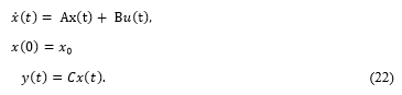
This paper deals with the control problem for nonholonomic wheeled mobile robots moving on the plane, and in particular, the use of a Fuzzy controller technique for achieving a given motion task which consists of following a rectilinear trajectory until an obstacle occurs on the path. After a background part, in which the fundamental knowledge of Fuzzy control is considered, the problem of the avoidance of an obstacle is taken into consideration. When an obstacle occurs on the path, the drive assistant provides for its avoidance calculating the minimal distance from which the avoidance maneuver starts. Conditions on the parameters of a PD controller are calculated using a Fuzzy based approach. An observer is designed to obtain unmeasurable states to be used in the control loop. In the Appendix of this paper a formal demonstration of a Proposition is proven in which the convergence of the system state estimation of the observer is shown. Simulations considering a real transporter vehicle for a storage service are shown.
1. Introduction
In the field of logistics, the demand for shorter lead times, the highest possible flexibility and high efficiency increases every year. In order to implement these requirements, it is of a great importance that the resources which are responsible for the flow of materials should be optimized and designed so that they can be intuitive and easy to be used. For transportation today as it was in the past, trucks and pallet trucks are used and it is essential to employ personnel for picking within the warehouse. Since a high potential for improving the picking process is still present, a high level of attention will be paid to the optimization of these tasks.
This paper is an extension of work originally presented in ICCC conference 2018, [1]. The difference between this work and that already published in [1] is a wide extension of the simulated results together with an extension of the background aspects related to the Fuzzy control and the Luenberger observer. Moreover, the demonstration of the convergence of the estimation is reported in the Appendix of this paper. In this sense, the problem of the observer is considered in depth because represents one of the most challenging problems. The idea is to control the vehicle using the measurement of the steering angular position and the position of the vehicle. The aim of this work is to create a simulation by which the evasive behavior of a newly developed Picking Vehicle can be tested. The results of this work can be applied at a later stage to a second stage of the vehicle. The simulation allows to test the vehicle’s behavior and it gives ideas for the design of the controller parameters. More in depth, this paper deals with the control problem for nonholonomic wheeled mobile robots moving on the plane, and in particular, the problem of the avoidance of obstacles is taken into consideration. When an obstacle occurs on the path, then the drive assistant provides for its avoidance calculating the minimal distance from which the avoidance maneuver starts. Using a Fuzzy approach, conditions on the parameters of a PD controller are calculated. A Luenberger observer is used in the control loop to minimize the number of the sensors. It is known that Luenberger observer is one of the most used observers in motion control and it is a high gain observer, see [2, 3] and [4] and Kalman Filters, see [5] and [6]. Even though the model of a mobile robot is well known in terms of its structure, for controlling mechanisms Fuzzy logic is often used, see [7]. The use of Fuzzy controller is not limited to the system without physical insights but it is shown in [8] that any system can take advantage from such a kind of control strategy. In particular, in [9] the authors describe the design and the implementation of a trajectory tracking controller using Fuzzy logic for mobile robots to navigate in the indoor environments. Most of the previous works used two independent controllers for navigation and avoiding obstacles. Also in [10] the salient feature of the proposed approach is that it combines the Fuzzy gain scheduling method and a Fuzzy proportional-integral-derivative (PID) controller to solve the nonlinear control problem. The paper is organized in the following way. Session 2 presents the model of a general nonholonomic system. Session 3 is devoted to the presentation of the Luenberger observer. Session 4 is dedicated to the Fuzzy and PD control strategy. Session 5 shows the simulated results and the conclusions close the paper. At the end of the paper in an Appendix, a Preposition is proven in which the convergence of the estimation of the system state variables is shown.
2. The Nonholonomic System
The first step in developing the kinematic model, which will be used below, is the consideration of nonholonomic conditions. The model used is that of robots with car-like properties. Therefore, the properties of the robot will be described by means of the position and the orientation of the vehicle along the route and the angle of the wheels to be controlled. The main feature of the mobile vehicle similar to a robot is the presence of nonholonomic constraints, since they are based on the condition of getting around without slipping on the ground. This means that the movements of the vehicle are restricted and the vehicle cannot move freely in any direction, see [11]. One example is the parallel parking a car. To get into the parking space it is not possible to drive the vehicle easily sideways. It must be moved forward or backward and be maneuvered by means of changing the steering angle of the front wheels into the parking space. To understand the conditions of the nonholonomic system, at the beginning the case of each wheel will be considered. The speed of the wheel is orientated in the direction in which the wheel moves.
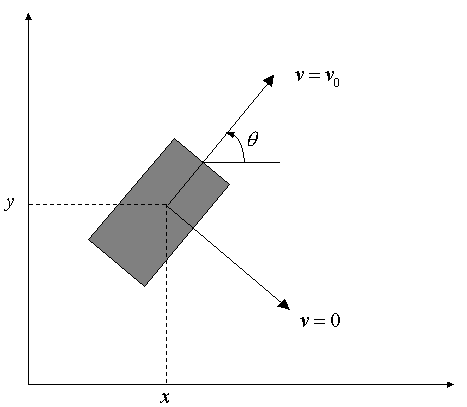 Figure 1. Nonholonomic system: (Mellodge, Feedback Control for a Path Following Robotic Car, 2002)
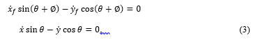
Due to the nonholonomic properties speed in other directions is not possible. The properties of each single wheel can be described using a vector consisting of three generalized coordinates. The position coordinates x, y within a fixed coordinate system in which the wheel touches the ground and the angle θ, which is the alignment of the wheel to the x-axis. The generalized velocities q cannot accept independent values, they are subject to the following constraint, see Figure 1 from [12]:
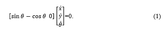 Equation (1) constitutes a particular expression of a kinematic constraint, a Pfaffian constraint. In this case, the Pfaffian , for example, is linearity in the generalized speeds. As a result, all the generalized velocities in the core of the matrix C (q) are included, see [13].
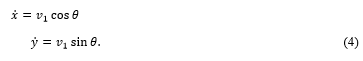
For the individual wheel, this results in the following model:
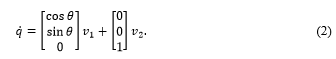 In this case, represents the linear speed of the wheel and represents the angular velocity around the vertical axis.
2.1. Kinematic Model of the Vehicle with Global Coordinates
The kinematic model of a vehicle is often used because of its simplicity and its accuracy when the vehicle behavior must be shown under normal driving conditions, see [14]. The model of a car-like robot vehicle is an option for the kinematic model. This can be described (see Figure 2) on the basis of four variables, see [14].
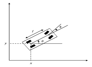 Figure 2. Car model with global coordinates (Source: (Mellodge & Kachroo, 2008), page 31)
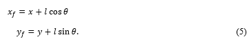
and represent the Cartesian coordinates of the rear axle of the vehicle. The angle θ is the orientation of the vehicle with respect to the x-axis and the angle ∅ which shows the steering angle of the front wheels of the vehicle, θ with respect to the alignment. Because of front and rear axles, the system is subject to two different nonholonomic conditions:
 where and represent the coordinates of the front axle, and represent the coordinates of the rear one. From the conditions shown in Figure 2, the current velocities in and directions can be calculated, in which represents the speed at the rear wheels:
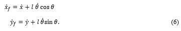
 Taking the rear axle as a reference point and taking into account the distance between the two axes, the result for the front axle is:
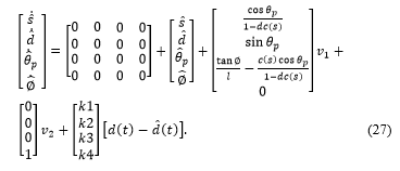
 This results in the position of the derivative to the speeds:
 If the new conditions of formula (2.6) in the nonholonomic conditions of the front axle (2.3) are used and solved for θ, then the constraint of the front axle results to be:
From this, the entire model results as follows, see also [15]:
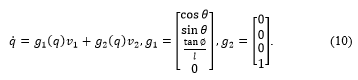
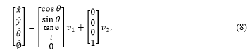 thereby represents the speed of the rear wheels and represents the speed of the steering angle or the change of the steering wheels. In order to investigate the nonlinear system from the previous equation, the principle of the Lie algebra provides the ability to perform a controllability analysis. The existing system is known to be a nonlinear and a drift-free one due to the nonholonomic conditions of the system. A general description of the kinematic nonlinear system is shown below in equation (9):
![]() Here, q represents the n vector of the general coordinates.
Here, q represents the n vector of the general coordinates.
is the m-vector of the input speeds, and it must be smaller than the amount of the general coordinates (m <n). The matrix G is divided into a plurality of uniform columns, where (i = 1, …, m) is valid. For the model of the vehicle like robot which is used, n = 4 different coordinates and m = 2 controllable inputs are valid. This results in the following model which is used for the consideration of controllability, see [13].
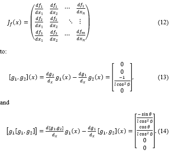
 The two vector fields and and allow driving and steering of the model. Apparently only the directions given by and are possible, but in reality, it is known that practically any position can be approached with a car. To describe the process mathematics provides the method of Lie derivative, which creates a new vector field out of two vector fields. In [12] the Lie brackets are designed as follows:
![]() The brackets and are already known, the other two arise by means of the Jacobian matrix:
The brackets and are already known, the other two arise by means of the Jacobian matrix:
 Further matrices are not present and therefore, the individual matrices can be merged to the overall matrix G. Finally, the rank of the matrix will be determined. Matrix G is the following:
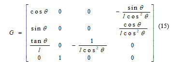 From the consideration of matrix G, the rank of this matrix results to be equal to four, because all four columns are independent for all θ. From the middle two columns it is directly visible that they cannot be zero. The two outer columns should be specifically considered, because of the danger that for ∅ = 0 a dependency can occur. For this, the determinant of the matrix G was calculated by the symbolic toolbox of MATLAB. This investigation showed that except in the case of a higher or lower steering angle of ∅ = ± π/2 there is no dependency. It follows that the system is controllable, as long as it is within the valid steering angle, see [5].
2.2. Kinematic Model of the Vehicle with Path Coordinates
The Global Coordinates model of the vehicle presented in subsection (3.1) is useful for the purpose of simulation and of good use to gain first insights into the behavior. However, for an application in practice, it is not particularly suitable in most cases because the sensors have difficulty to determine the position of the vehicle in relation to global coordinates. Therefore, a new model must be introduced for the rest of the work. This describes the position of the vehicle as dependent of the path (Figure 3). The distance, which the vehicle must keep to the wall and to obstacles is indicated by the variable and measured by the laser scanner, which is located centrally on the vehicle front side. The distance between the front and the rear axle is defined by l. The angle θ reproduces the orientation of the vehicle with respect to the x-axis again as also in the global coordinate system. indicates the angle between a tangent to the path and the x-axis. In order the vehicle to be able to follow the path, an angle which indicates the difference between the orientation of the vehicle and the angle of the tangent is defined:
![]() For the desired path, tracking this difference should tend as much as possible to zero. The distance traveled is defined by s and is an arbitrarily selectable starting position. The course of the track, or for instance, the curvature is given by c (s) and defined as follows:
For the desired path, tracking this difference should tend as much as possible to zero. The distance traveled is defined by s and is an arbitrarily selectable starting position. The course of the track, or for instance, the curvature is given by c (s) and defined as follows:
![]() Furthermore, the speeds along the track and the speed required perpendicular to the distance for the model will be required:
Furthermore, the speeds along the track and the speed required perpendicular to the distance for the model will be required:
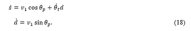
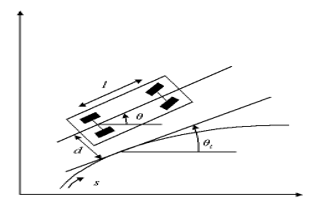 Figure 3. Kinematic Model with Path coordinates (Source: (Mellodge & Kachroo, 2008), page 33)
The overall model based on the redefined variables with Path Coordinates, as it can be seen in Equation (19), can be set up.
 3. Observer
The state variables must be supplied to the controller for the control of dynamic systems or control of the physical parameters of the track. These quantities are usually measured. However, if this is not possible, or only possible with a great effort, they have to be determined in another way. For this, an observer can be used, which reconstructs a state (condition) based on the course of input and output variables. Here, the model of the controlled system is connected in parallel to the actual process and supplied with the same input dimension. If the model is correct, it performs the same action as the control path and differences can thus only occur through the different initial conditions. If the control system is stable and it is possible to wait long enough, the observer and the controlled system commute into the same sizes and it is: and and can be used as a state feedback. This simple variant has major lacks:
- The control path will only consider a disturbance size, while the model remains unchanged, when a disturbance occurs. Therefore, this method is only suitable for undisturbed, uninteresting cases for control.
- Secondly, a difference generated by different initial states and is only compensated when the controlled system is stable. Out of the equation of the state of the controlled system:
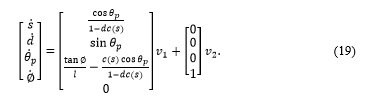
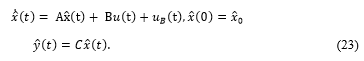
This however is only possible for a stable matrix A against zero, regardless of whether the unstable controlled system is stabilized within the control loop by a state feedback. Since only the system matrix of the controlled system and not of the closed circuit enters into the relationship, the simple observer is useful only for stable systems. Based on this principle, David G. Luenberger has developed an extension of this model in 1964. However, this observer is expanded to the difference between the output of the model y and the output of the control path y. This difference is used in order to equalize the state of the model to the route. This method has already proven itself in the control loop, there, however, the deviation of the controlled variable is used to perform a control intervention, which influences the controlled variable. Based on the following non-jump-capable control system the subsequent design of the observer follows:
 In the design of the observer, the system model is supplemented by the input :
 In the new input the difference between the measured output of the control path and the output of the model is returned to be:
![]() If equations (3.4) and (3.5) are put together, we obtain the following relationship:
If equations (3.4) and (3.5) are put together, we obtain the following relationship:
![]() After merging, the effect of the newly introduced input is recognized. As long as is true, the right part falls away, because the addend becomes zero and the model thus runs in parallel to the control path. If a deviation between the input variables, which influence the outputs, occurs, so the behavior of the model due to the feedback will be influenced. In order to reduce the deviation, a matrix L must be found which decreases the difference of . The input vector is not known in practice as a rule, however, the output vector , serving as an input of the observer. The result for the observer is a controlled dynamic system with the two inputs u(t) and y(t) as in equation (3.7).
After merging, the effect of the newly introduced input is recognized. As long as is true, the right part falls away, because the addend becomes zero and the model thus runs in parallel to the control path. If a deviation between the input variables, which influence the outputs, occurs, so the behavior of the model due to the feedback will be influenced. In order to reduce the deviation, a matrix L must be found which decreases the difference of . The input vector is not known in practice as a rule, however, the output vector , serving as an input of the observer. The result for the observer is a controlled dynamic system with the two inputs u(t) and y(t) as in equation (3.7).
![]() In the simulation, the observer has the following characteristics:
In the simulation, the observer has the following characteristics:
 The principle of the Luenberger observer is based on a linear system, in which matrices with fixed values are integrated. However, the system in the work is a nonlinear one, in which the matrix B represents a field with variables. The principle of the observer remains the same as the one in the linear version. The stability of the observer seems to be given, however, it was only heuristically determined. To investigate the stability more precisely, the stability theory of Lyapunov is used and in the Appendix at the end of the chapter a formal analysis is conducted.
4. Fuzzy Control Algorithm integrated with a PD controller
In addition to methods for mathematically analytical problem solving of control and monitoring tasks, now human experience and knowledge that cannot be expressed mathematically for problem solving are being increasingly used. For this purpose, the Fuzzy logic is often used. In contrast to the classical control engineering, the behavior of a system is tried to be described with traditional means and then a controller will be tried to be designed with analytical methods. Fuzzy systems are particularly well suitable for the design of systems under a vague knowledge. For example, they are well suitable for not exactly known process or a not exactly known controller behavior. Due to the completely different approaches for both controller designs, completely different solution approaches for Fuzzy and classical approaches for regulation are used. While in the classical, for instance PD scheme, in a first step a model of the controlled-track is formed, in the second step the associated controller design follows only using the formed path. This procedure can therefore be described as a model-driven interpretation. The Fuzzy controller represents a contrast for it, since, this is controller-oriented. Subsequently, the basic concepts of Fuzzy control, and the steps of the design of a Fuzzy controller are described. For execution of the control mechanism in Fuzzy logic three actions must be performed. In the first part, the sharp values, which are supplied by the input variable, will be transformed into the fuzzification. The physical values of input values become the converted Fuzzy sets. These are a specific form of Fuzzy sets, in which the values are not described as usually in mathematics by numerical variables in the form of sharp numbers, but by colloquial expressions. Here formulations arise such as: when the distance to the wall is too small, the distance must be increased somewhat by increasing the steering angle. Here, the descriptions “distance slightly too small” and “steering angle slightly increase” represent the blurry relationship between the distance to the wall and the steering angle. The variables, which result from this, are called linguistic variables and they will be assigned to a membership function. The membership function makes an indication, in what proportion between 0 and 1, the value of a blurry statement is true. It also provides a statement to what extent an element belongs to a certain set. In literature fuzzy controller is used also for nonholonomic systems. In [16] a fuzzy PD controller for a dynamic model of nonholonomic mobile manipulator in order to treat the trajectory tracking control and to eliminate the effect of external force on the end-effector is proposed. Concerning the robustness of the Fuzzy approach, the paper in [17] addresses the output feedback trajectory tracking problem for a nonholonomic wheeled mobile robot in the presence of parameter uncertainties, external disturbances, and a lack of velocity measurements. A combination between a heuristic Fuzzy and PID controller is also designed in [18] to move the robot upward or downward the inclined plane and approach the target point. In [19] fuzzy adaptive observers together with parameter adaptation laws are designed to estimate the state-dependent disturbances in both kinematics and dynamics in order to adapt a Fuzzy adaptive controller.
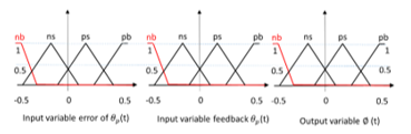 Figure 4. Top left: input variable error of ; top right: input variable feedback ; bottom left: output variable ∅; bottom right: overall structure of the Fuzzy controller
In [20] a holistic, for holonomic and nonholonomic systems, intelligent control strategy is proposed in which only position measurements are used.
In Figure 4, the two inputs and the output of one of the two Fuzzy controllers are presented as an example. Here the different Fuzzy sets of the two inputs and the output can be seen. The linguistic variable “ns” means “negative small” and is associated with an interval 0.1 to -0.4. Within the interval there are different degrees of association, the value 0.15 with a factor of 1 is the most strongly associated value and the association decreases in negative and positive direction until at 0.1 and -0.4 the association of 0 is achieved. Such linguistic variables are defined over the entire area to be controlled, if possible, they must have an overlap at their adjacent variable, so that no areas remain undefined. In order to provide a high degree of flexibility in different executions such as trapezoidal, Gaussian, or triangular shaped, the associated functions can be defined and combined with each other. MATLAB provides for different execution forms. In the present work, the trapezoidal and triangle-shaped execution have been chosen.
Table 1. Fuzzy rules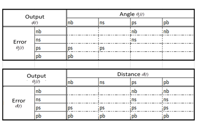
In Table 1 all the used fuzzy roles in this application are indicated. For instance, the linguistic variable “nb” stands for “negative big,” “ps” stands for “positive small” and “pb” stands for positive big.
After the fuzzification was performed, the inference follows. The rules for evaluation will be developed with help of an expert or by a private experience. These consist of two parts, the if-condition (premise): IF the distance is too small and the Fuzzy inference (conclusion): THEN the steering angle must be increased slightly. The input variables will be linked by means of an AND-operation in the IF part. Then the resulting rules are connected by means of an OR-operation. So, the following rules resulted for the conditions used in this work. The possible Fuzzy sets for the deviation from the desired value are referred here as an error. The Fuzzy sets that are delivered as a response of the system, are referred to as a feedback. A 4×4 matrix follows from it, in which not every field is filled. The actual inference takes place within three steps after the rules having been defined:
- Aggregation (evaluation of the rule premises): The rule premises are evaluated here, that is the IF-parts of rules corresponding to their affiliations and selected operators. The input variables were associated with an AND-operator, in this case a min-operator results to be used, which always selects the smallest affiliation value of a Fuzzy set. From a human point of view, it acts pessimistically and not compensatory.
- Implication (evaluation of the conclusions (THEN-part)):
Evaluation of the conditions occurs during the implication. The rules can also only be partially true in the Fuzzy control, in contrast to the classical control. Therefore, in this step, a definition follows in which the dimension of the condition is true or not. The minimum procedure will be used for it (see Figure 5), which assumes as a conclusion the minimum of the premise (IF-part) and conclusion (THEN- part). In simple words, this means that the output function as a result of this operation, is cut off at the level of fulfillment of the premise and an area in the output Fuzzy set arises.
- Accumulation (summary of all rules); The conclusions of all the rules will be summarized in the accumulation. This is necessary because, as a rule not only one rule is true, but several rules can be at least partially valid. Due to the fact that the rules are connected with each other through the Or-links, here the maximum operator is used in the selection of the conclusions. Here the maximum value of the Fuzzy sets is used as the output function, see Figure 6. Since the Min-method was used for the implication and the Max-method was used for the accumulation, the process which is applied in the work is called a max / min inference.
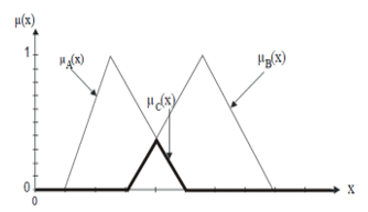 Figure 5. Minimum Operator
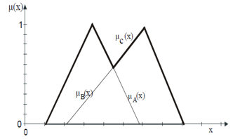 Figure 6. Maximum Operator
DE fuzzification is carried out during the last step, after the inference was completed. A new Fuzzy set will turn out to be from the inference, and thus a Fuzzy information will be delivered. So that other participants can process the signals, sharp output values must be generated again. This is done using the gravity method. Here, a Fuzzy set resulting from the inference is considered as a totality.
As shown in Figure 7, the Fuzzy set became a set B* which determines the output variable. The centroid is now determined by the gravity method and the gravity coordinate us gives it as a DE fuzzification result. The coordinate of the centroid is calculated by the following formula:
= sharp output value
= abscissa bases
= membership degree for
number of abscissa bases
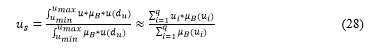
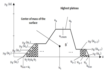 Figure 7. DE fuzzification by the centroid method (centroid)
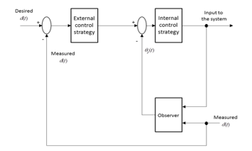 Figure 8. Simplified diagram of the cascaded control loop
During the calculation according to the gravity method, all active rules determine the sharp output. The calculation methods and criteria for the selection of operators are selected in Simulink within the Fuzzy Editor and run subsequently automatically.
Figure 8 shows the general structure of the cascade control scheme including the Luenberger observer. In Figure 8 it is visible how the observer is issued. Through the measurement of the distance between the car and the wall all other state variables can be observed.
Here, the outer and the inner circle of the PD and the Fuzzy control with help of an adder were interconnected. This is shown in Figure 9.
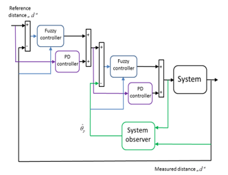 Figure 9. Simulink diagram combining PD and Fuzzy controllers in a cascade control structure together with an observer
The choice of this particular Fuzzy logic is due to the fact that, considering more variables than proposed, not relevant improvements are obtained in terms of reduction of error.
4.1. A Gaussian Curve to Avoid Obstacle
A Gaussian function offers the possibility to obtain the highest possible, incremental and without jumps resulting function to avoid obstacles. This guarantees due to its properties, in addition to a slow and continuous adjustment of the steering angle, a high degree of stability in its derivation. This property proves to be of a great advantage, because the derivative is required for further calculations within the simulation. To achieve a high degree of flexibility and influence a formed function, which is similar to a Gaussian function, but offers more free parameters, and thus becomes a Gaussian-like function. The calculation is based on the freely selectable amplitude H, which determines the maximum level of the function. In order to influence the abdomen of a function, upsetting or a stretching factor was introduced. This will be automatically calculated based on the obstacle width in a sub-function. The following formula is a result for the curve:
H = amplitude of the curve
o = factor for upsetting or stretching of the curve
t = velocity factor
![]() The derivative of the curve is thus obtained as follows:
The derivative of the curve is thus obtained as follows:
![]() Factor “t” states, in this case, the speed of the vehicle and the phase shift, which serves as a correction factor. In the following part the overall configurations of the various control concepts and their implementation in Simulink were presented.
Factor “t” states, in this case, the speed of the vehicle and the phase shift, which serves as a correction factor. In the following part the overall configurations of the various control concepts and their implementation in Simulink were presented.
5. Results
Figure 10 shows that the cascade PD control structure increases significantly faster the distance to the wall than the other two control configurations. This requires only 8 seconds, in the meantime the cascade Fuzzy control structure, represented in Figure 11, requires about 12 seconds to bring the vehicle at the same distance. The combination of both controllers manages to do it in just over 10 seconds, see Figure 12. During the fallback procedure, which starts at about 25 seconds, the quality of the results of the controller changes, the PD controller shows here his weakness. In the case of the example shown, this operation supplies during the evacuation process the worst results. It swings at the desired distance from ≈∓ 6 cm. The Fuzzy Control System in comparison provides results of ≈∓ 5 cm, which accounts for a difference of ≈17%. The combination of the two controllers presents the best results. This results in a maximum deviation of ≈∓ 2 cm, which means a difference of ≈67% compared to the PD controller. Thus, the combination of the two controllers in the simulation provides the best results, although it increases the distance to the wall something slower than the PD it performs, but it has a significantly higher stability during the fallback procedure. It is important to be able to configure the smallest possible protective field because the aisles in which the vehicle should move anyway already offer little space and thus the smallest possible protective field is necessary. A comparison between the model of the kinematic system and the estimated values of the observer based on the distance d is also visible.
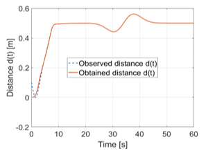 Figure 10. Distance of the car from the wall using the cascade PD control structure
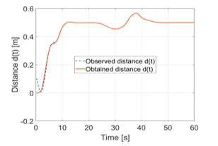 Figure 11. Distance of the car from the wall using the cascade Fuzzy control structure
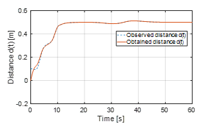 Figure 12. Distance of the car from the wall using the combination between PD and Fuzzy cascade control structure
To ensure that the vehicle does not slip during the evacuation process even with a heavy load, or does not even lose some of the load and also to be able to configure a minimum possible protective field, the steering angle may not exceed a maximum impact of ∓ 10°. Figures 13, 14 and 15 show the time progress of the steering angle in degrees using PD, Fuzzy and a combination of PD and Fuzzy controllers respectively. As it can be seen there, the requirement of the maximum steering angle has been met for all three schemes.
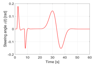 Figure 13. Steering angle ∅ using the PD cascade controller structure
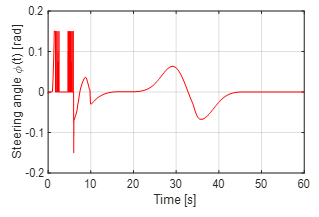 Figure 14. Steering angle ∅ using the Fuzzy cascade controller structure
However, it was shown that the PD control with ∓ 10 °, during the evasive maneuver, is still within the required range, but the other two controls are significantly lower. Thus, during the evasive maneuver, the Fuzzy control with a range of ≈∓8 ° and the combination of both controls, PD and Fuzzy controllers, lead the comparison with a range of ≈∓6 °. As it has already been described, also the combination of the two controls leads if we compare the simulation results, because it requires the least amount of the steering angle. Advantages of this are, as it has already been explained above, that no abrupt changes of direction as a result of a strong steering maneuver occur due to the small steering angle and the avoidance maneuver has fewer risks like slippage of the vehicle, or a shifting or falling down of the load. Figures 13, 14 and 15 show the simulation results concerning these aspects.
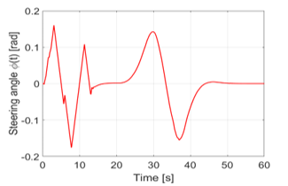 Figure 15. Steering angle ∅ using the combination between PD and Fuzzy cascade control structure
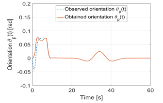 Figure 16. Angle using the PD cascade controller structure
5.1. Results of the Vehicle Orientation
The vehicle as it is described must follow the predetermined path. For this purpose, the differential angle was introduced which describes the difference between the angle to the path and the actual vehicle heading . Figures 16, 17 and 18 show the time course of the difference angle expressed in degrees. For the route to follow this best, the difference angle must be kept as small as possible. The initially large deflection is due to the correction, in order to achieve the already mentioned predetermined distance and in this case, less relevant, since this is not to be taken into account for the actual viewing of the path. Interestingly, the course is between 20 and 50 seconds since the avoidance of the obstacle occurs, which goes along with the path. Here, PD and Fuzzy controllers deliver almost equivalent results, but the maximum excursions hardly differ so they both achieve maximum angle of ≈∓1.5° during the evasive maneuver. It is different with the result of the combination of the two schemes, this is as well as the distance and the steering angle significantly better. Here is a maximum angle of ≈∓ 0.5° during the evasive maneuver and thus the best result. A comparison between the model of the kinematic system and the estimated values of the observer based on the angle is also visible.
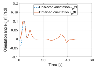 Figure 17. Angle using the Fuzzy cascade controller structure
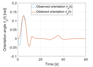 Figure 18. Angle using the combination between PD and Fuzzy cascade control structure
Figure 19 shows the error of the distance and Figure 20 shows the error of the orientation of the car. In both cases it is possible to see how after 45 seconds the error results to be almost equal to zero.
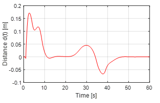 Figure 19. Error of the distance of the car from the wall
To discuss the obtained results with the already existing contributions it is possible to say that in this contribution an original combination of Fuzzy control strategy combined in a PD controller in a cascade structure is presented. This idea is an original one, which is not present in the already existing literature as already discussed through the cited literature.
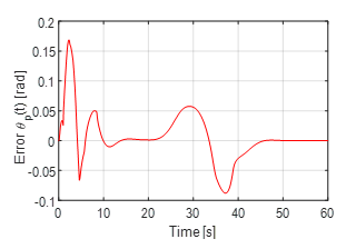 Figure 20. Error of angle
6. Conclusions
This paper deals with the control problem for nonholonomic wheeled mobile robots moving on the plane to avoid obstacles. Parameters of a PD controller are calculated using a fuzzy based approach. To estimate the orientation of the vehicle a Luenberger observer is involved in the control scheme. In the context of the Luenberger observer, the demonstration of the convergence of the estimation of the proposed observer is shown in the Appendix of the paper. Simulations considering a real transporter vehicle for a storage service are shown.
- P. Mercorelli, “Fuzzy based control of a nonholonomic car-like robot for driveassistant systems”, 2018 19th International Carpathian Control Conference (ICCC), Szilvasvarad, pp. 434-439, 2018.
- P. Mercorelli, “An adaptive and optimized switching observer for sensorless control of an electromagnetic valve actuator in camless internal combustion engines”. Asian Journal of Control, 16:959–973, 2014.
- P. Mercorelli, “A two-stage sliding-mode high-gain observer to reduce uncertainties and disturbances effects for sensorless control in automotive applications”. IEEE Transactions on Industrial Electronics, 62(9):5929–5940, 2015.
- P. Mercorelli, “A motion-sensorless control for intake valves in combustion engines”. IEEE Transactions on Industrial Electronics, 64(4):3402–3412, 2017.
- P. Mercorelli, “A two-stage augmented extended Kalman filter as an observer for sensorless valve control in camless internal combustion engines”. IEEE Transactions on Industrial Electronics, 59(11):4236–4247, 2012.
- P. Mercorelli, “A hysteresis hybrid extended Kalman filter as an observer for sensorless valve control in camless internal combustion engines”. IEEE Transactions on Industry Applications, 48(6):1940–1949, 2012.
- C. Zheng, Y. Su, P. Mercorelli, “A simple fuzzy controller for robot manipulators with bounded inputs”. IEEE/ASME International Conference on Advanced Intelligent Mechatronics, AIM, 737–1742, 2017.
- G. Feng, “A Survey on Analysis and Design of Model-Based Fuzzy Control Systems”. IEEE Transactions on Fuzzy Systems, 14: 676-697, 2006. doi: 10.1109/TFUZZ. 2006.883415.
- H. Omrane, M. S. Masmoudi, M. Masmoudi, “Fuzzy Logic Based Control for Autonomous Mobile Robot Navigation”, Computational Intelligence and Neuroscience, 2016, Article ID 9548482.
- Y. L. Sun, M. J. Er, “Hybrid fuzzy control of robotics systems”, IEEE Transactions on Fuzzy Systems, 12: 755-765, 2004. doi: 10.1109/TFUZZ.2004.836097.
- F. Fahimi, Autnomous Robots Modeling, Path Planning, and Control. New York: Springer Science & Business Media, 2009.
- P. Mellodge, “Feedback Control for a Path Following Robotic Car”. M.S. Thesis, Blacksburg: VirginiaTech, 2002.
- J.-P. Laumond, Robot Motion Planning and Control. London: Springer, 1998.
- P. Mellodge, K. Pushkin, Model Abstraction in Dynamical Systems: Application to Mobile Robot Control. Berlin Heidelberg: Springer, 2008.
- A. De Luca, G. Oriolo, C. Samson, “Feedback control of a nonholonomic car-like”. In Jean-Paul Laumond, editor, Robot Motion Planning and Control, 4: 171–253. Berlin Heidelberg: Springer, 1998.
- A. Karray and M. Feki, “Tracking control of a mobile manipulator with fuzzy PD controller”, 2015 World Congress on Information Technology and Computer Applications (WCITCA), Hammamet, pp. 1-5, 2015.
- S. Peng, W. Shi, “Adaptive Fuzzy Output Feedback Control of a Nonholonomic Wheeled Mobile Robot”, in IEEE Access, vol. 6, pp. 43414-43424, 2018.
- M. Roozegar, M. J. Mahjoob, “Modelling and control of a non-holonomic pendulum-driven spherical robot moving on an inclined plane: simulation and experimental results”, in IET Control Theory & Applications, vol. 11, no. 4, pp. 541-549, 24 2, 2017.
- D. Chwa, “Fuzzy Adaptive Tracking Control of Wheeled Mobile Robots With State-Dependent Kinematic and Dynamic Disturbances”, in IEEE Transactions on Fuzzy Systems, vol. 20, no. 3, pp. 587-593, 2012.
- Y-C. Chang, B-S. Chen, “Intelligent robust tracking controls for holonomic and nonholonomic mechanical systems using only position measurements”, in IEEE Transactions on Fuzzy Systems, vol. 13, no. 4, pp. 491-507, 2005.
- G. Zhu, A. Kaddouri, L. A. Dessaint, O. Akhrif. “A nonlinear state observer for the sensorless control of a permanent-magnet ac machine”. IEEE Transactions on Industrial Electronics, 48(6):1098–1108, 2001.