1. Introduction

The main challenges affecting today’s Supply Chains (SCs) are globalisation, environmental and technological turbulences and rapid changes in economy capacity. They have provoked companies to recognise that, in order to remain competitive in the global market, they need to gain more from their SCs.

Supply Chains are defined as links (relationships) between every unit (enterprise) in a manufacturing process from raw materials to customers. Traditionally, products were made and flowed to consumers through SCs. However, due to globalisation and complexity of the economy, today’s SCs are better characterised as Supply Networks (SNs).

Consumer Supply Networks (CSNs) refer to complex networks consisting of sets of companies working in unison to supply, manufacture, distribute and deliver final products and services to end-users (Figure 1), being controlled by information flow.

CSNs are examples of industrial systems that are naturally large, complex, stochastic, and dynamic. These attributes translate into difficulties in representing the actual behaviour and in planning, optimising and anticipating performance. Also, the combination of these attributes makes the choice of an appropriate solution methodology difficult at best, if not simply impossible at this point in time [1].

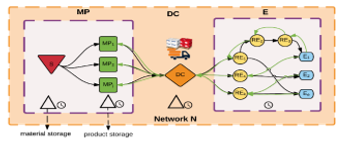Figure 1  Three echelon Consumer Supply Network

Different methodologies have been utilised to solve this class of complex problem; simulation and optimisation methods are widely used to tackle such problems.

Simulation is a powerful tool for modelling, analysis, and validation of CSNs. However, its major disadvantage is that it will produce a very detailed analysis but strictly for a given configuration. Simulation cannot change the configuration of the system, and any optimisation would be searching for the best combination of variables for a given system.

A recurrent, key issue when attempting to optimise CSN is the granularity of the model. An appropriate granularity – the size of the smallest indivisible unit (of product, part, flow, time, etc.) of the process – makes the difference between a successful implementation of the optimisation methodology and an algorithm that does not converge or gets consistently stuck in local optima. Additionally, the choice of the granularity of the model has to be easy to translate in practice – a purely theoretical solution that cannot be implemented in real life is of little help.

This paper is an extension of the work initially has been presented in Intellisys Conference [2] in which a unique simulation optimisation approach (SOA) within an integrated methodology was developed. A small-scale Multi-Period, Multi-Product Consumer Supply Network (MPMPCSN) model, using mixed integer non-linear programming (MINLP) was designed. Then, the optimum quantity of orders was determined incorporating GA optimisation algorithm which simultaneously results in the total inventory cost minimisation. This way, the unique advantages of simulation were incorporated with optimisation method and higher quality solutions were achieved. Also, the quality of the solutions that were obtained by the proposed framework was checked by fine-tuning of the search algorithm’s parameters combining the simulation model with the Taguchi method. Hence, in this study, a series of computational trials on realistic test problems are designed and analysed to demonstrate the generalisability of the proposed SOA for problems of similar size at different granularity levels.

The rest of this article is organised as follows: Section 2 is devoted to reviewing modelling methodologies that were used to solve CSNs problems. Section 3 presents the proposed MINLP model. Section 4 provides details about granularity. The optimisation module of the SOA methodology is described in Section 4. The numerical examples are given in Section 6 and discussed in Section 7. Section 8 concludes the paper.

2. Literature Review

A number of potential solution methods for the class of problems of similar size and complexity have been developed in the literature ranging from classical mathematical programming to hybrid and systematic methods [1, 3].

Optimisation methodologies combined with mathematical models are mainly contributed to solutions validation. A stable optimal solution can be obtained by a given objective function subject to several constraints. However, they are unable to provide the gradient of design space over time [4]. The extent of the optimisation problem cannot be expanded beyond a certain limit as the complexity of the problem adversely affects the computational costs which make less efficient and less practical [5]. This concern can be addressed by using, simulation methodologies.

Simulation models can deal with all attributes of CSNs problems which makes them a powerful analytical tool in this area [6]. In particular, CSN simulation provides a model that suitably represents, processes associated with specific business units such as ordering system, manufacturing plant, distribution centres, etc. in the presence of uncertainty [7, 8]. Simulation modelling methods alongside with mathematical and models based on algorithms almost always come together. The main advantage of simulation approaches is a possibility to explore what-if scenarios that provide a deeper understanding of the dependencies in a system. The operations of a real system that are usually very dangerous, expensive, or impractical to implement can be evaluated according to their resilience and robustness subject to various predefined inputs (e.g. time horizon, resources, etc.) and at any desired granular level via simulation modelling. Using computer programming, the performance of a real system subject to controlled and environmental changes can be simulated. Therefore, many input values and their combinations can be explored through simulation models [9]. Also, simulation models offer flexibility in developing and assessment of different scenarios, with reasonably high-speed processing. In addition, an embedded standard reporting system make them unique in modelling, analyzing, and validating of complex systems.

As pointed out, independent deployment of optimization and simulation methodologies has some benefits. However, it also has limitations. The main drawback of simulation models is that they can only work with a set configuration of a solution. On the other hand, finding the optimal solution by independently using the traditional optimization approaches incurs heavy computational cost. Therefore, the integration of the two methods may lead to a uniquely efficient optimization.

SOA is a key factor of modern design across industries [3]. SOA is often used in the design, modelling and in analyses of systems. It can provide an optimal setting for set of parameters for a simulation model [10]. But due to high computational requirements, scientists have not given much attention to the use of SOA in CSNs [10-12]. Consequently, SOA turns into a hot research topic for optimization of CSNs. The optimization core together with a simulation model in SOA, can search the solution space globally (ergodicity of GA) whereas the simulation module acts as a quality assessment unit.

Following the advances in computational power, increased efforts have been made to leverage simulation for optimization/simulation-based optimization of hybrid systems with behaviors that can be discrete or continuous [13]. CSNs are hybrid systems with a high level of complexity.

Inventory control planning problems have been tackled using many metaheuristic algorithms [5, 14-18]. GA was widely used to solve related problems [19]. Through exploring the solution space, GA finds optimal or near optimal solutions. But, like in other evolutionary algorithms (EA), GA cannot carry out self-validation. GA risks to converge to local optima [20]. Hence, a valid question is whether or not the obtained solution is a high-quality candidate.

The parameters of the search algorithm – population size, crossover and mutation and rates, as well as the interaction between these parameters have significant impacts on the quality of solutions. As the entire search population or its fitness function might be highly affected by variation of these parameters. This necessitates implementation of a mechanism that can offer parameters tunning is essential. However, it is very hard to perform perfect tuning due to complexity among the interactions of EA’s parameters. Most often, trial and error of EA’s parameters is used in OR studies. However, experimentally tuning the parameters is less practical and very expensive [21]. We thus, propose using statistical methods based on experiments as a more robust approach [22].

In [23], the authors present a multi-echelon SN simulation-based optimisation model for a multi-criteria P-D design. The model offers concurrent optimisation of the network’s structure, the set of the control strategies, and the quantitative parameters of the strategy for control. The modelling, simulation and then optimisation of networked entities are performed using a graphical interface designed in C++ programming. In this study, the candidate solutions are evaluated by a discrete-event simulation (DES) module. A multi-objective GA algorithm is developed aiming at finding compromised solutions regarding structural, qualitative and quantitative variables. The toolbox developed in the research considers a real Production-Distribution model which makes it a unique decision support system. However, there is no evidence shown with regards to parameters tuning of the GA algorithm.

In [24], the authors describe a two-phase Mixed Integer Linear Programming model addressing planning and scheduling systems of a build-to-order SN system. They use GA to optimise the aggregate costs of both subsystems. Three different scenarios were developed, in which distinct recombination rates for genes was used to improve the quality of solutions.

In [25], the researcher model a P-D network over a tactical planning horizon with uncertain demands and capacity. The proposed algorithm incorporates a simulation and an optimisation module; each calculates the total costs of the network for P-D. The problem is mathematically formulated by a MILP, and the fitness function (total cost) is evaluated via the simulation core. Then the solution resulting from the optimisation module is compared with the obtained output from the simulation module recursively. This procedure iterates until there is a set difference between two solutions. This study reports on data obtained from the implementation of the proposed SOA on a SN problem of a reduced scale. Although the simulation and the optimisation modules are both included in the proposed approach, there is no interaction or connection between them. The application of the simulation module is used to produce initial values for the parameters of the mathematical model. Also, the capacity to generalise the model for similar or larger problems was not addressed. Moreover, no evidence was shown around approaching a solution with better quality if different configurations were chosen for the optimisation parameters.

In [15], the authors developed a modified Particle Swarm Optimisation model (MPSO) for a location-allocation Supply Network problem. They formulated a two-echelon Distribution Network (DN) considering multi-product and multi-period inventory, subject to uncertainty of seasonal demands. The determination of the orders quantity and the vendors’ location are pursued as the main objectives in this paper. They use Taguchi to tune the parameters of the MPSO. They considered parameter tuning in their model and they performed a sensitivity analysis for similar problems with different granularity levels.

In a similar study, In [26], the researcher developed a PSO algorithm attempting to find the maximum profit for a channel of a two-echelon SN for a single product. Sales quantity and production rate were used as decision variables of their model. Using a combination of GA, PSO, and simulated annealing (SA), they conduct a detailed sensitivity analysis. However, the improvement of the proposed heuristic is computed by using another heuristic. This seems very inefficient.

In [27], the authors proposed a simulation optimisation approach to reduce the number of delayed customer orders while costs are kept under control for an integrated production-distribution supply chain. The hybrid modelling combined linear programming and discrete event simulation. This research is a great potential of using SOA approach; however, no effort was made considering the tunning of the control factors of the GA algorithm.

In [28], the researchers developed an agent-based simulation optimisation model through which an online auction policy within the context of the agricultural supply chain was optimised. Three different scenarios namely, oversupply, balance and insufficient supply with different demand and supply quantities were presented to obtain the optimal lot-size and to determine the optimum online auction policy to control inventory. The investigation towards improving the solution quality derived from the proposed methodology was not provided.

An important observation concerning SOA studies is that, in almost all studies, the tuning of the model’s variables (e.g. lead time, production rate, etc.) was only attempted in the optimisation module for small problems. Good examples are included in [20] and [22]. On the other hand, evidence in this regard seems to be missing in some studies [23, 29]. Furthermore, very few ([15, 24]) indicated efforts for tuning the optimisation parameters – selection methodology, mutation, and crossover in GA or swarm’s cognitive and social components in PSO. They reported that this had been done by trial and error – a typical approach used in the majority of OR studies [21]. The simulation model is run several times, then the better solution is selected. Due to the complexity of the interaction of parameters of the search algorithm as well as the high computational cost, it is unclear how many iterations would be sufficient for a given size problem. Besides, as the scale of the problem increases, the complexity of interactions increases exponentially. Therefore, the difficulties corresponding to this class of SNP problems will further escalate if a more detailed model is simulated. So, it is necessary to study in more depth the variation of the solution quality.

This paper presents an integrated simulation-optimisation approach to solve a class of CSN problem using GA. The objective is to minimise the total cost while an optimum/near optimum inventory level associated to each product family is obtained. An important feature of the under-investigated problem is that both demand and the inventory capacity are uncertain. The randomness of the uncertain parameters is captured by the simulation model. The optimal quantities are searched by GA. Also, a fine-tunning mechanism for the optimization algorithm’s controllable parameters is applied using Taguchi experimental design and ANOVA to improve the quality of the solution. In Section III, the mathematical model, parameters and notations of the proposed problem are summarized.

3. Mathematical Model

This section presents a mathematical model for a multi-product multi-period consumer supply network. The mathematical model presented here consider a planning period of T (indexed by t), a set of product family P (indexed by i) and a set of retailers R (indexed by j) with the limited budget and inventory restrictions.

The parameters in the model are the following:

	Demand for product family  by retailer  in period
	Demand for product family  by retailer  at the end of period
	Initial inventory level for product family
	Minimum quantity of product family  manufactured for retailer  in period
	Maximum quantity of product family  manufactured for retailer  in period
	Maximum capacity of the inventory at DC
	Total capacity of inventory at DC in period
	Cost for the ordering of product family
	Cost for purchasing one unit of product family at time
	Storage cost for one unit of product in period
	Handling cost at DC for one unit of product family in period
	Cost for backordering one unit of product family in period
	Cost for transporting one unit of product family in period
	Total cost of ordering at the end of period
	Total cost of storage in inventory at the end period
	Total cost of handling in inventory at the end of period
	Total cost of purchasing at the end of period
	Total cost of order shortage at the end period
	Total cost of transportation at the end of period
	The total network costs at the end of period
	The backorder intensity rate for product family  at the end of period
	The capacity severity rate for product family  at the end of period

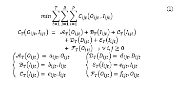
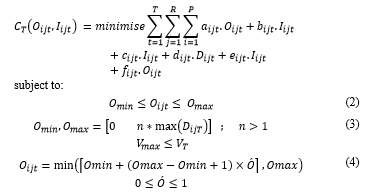
The objective function (1) comprises the minimization of the total CSN costs, consisting of ordering costs, purchasing costs, transportation costs from manufacturing plants (MP) to retailers (RE), inventory holding and handling costs at the distribution center (DC), and backordering costs subject to a set of constraints present in (2-4). Constraint (1) represents the quantity of order of a product family  in a period  bounded by the upper and the lower limits. Note, the maximum quantity of an order for product family  from retailer  cannot exceed maximum  folds of the maximum quantity of the demand for the entire planning period . Constrain (2) is the capacity of the inventory denoted by . The order quantity is a positive integer that is normalized between 0 and 1 by (4) denoted by . Table 1 and Table 2 shows a numerical representation of  and  for , 5 and  .

• numerical representation of

Note:  presents the quantity of product family 1 to be manufactured for consumer 1 in time interval  is 259 unit.

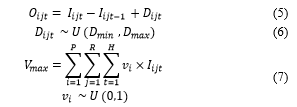
The  and are related to the decisions regarding the inventory level and the quantity of orders that are calculated by (5).  is the main decision variable, since is obtained recursively from . The demand quantity,  is unknown but bounded. It can be expressed by probabilistic distribution functions such as normal or uniform distribution functions. In this model, a uniform distribution is used to model  using (6), where  are the lower and upper bounds, respectively.

Also, each product family has a set volume ( ) so the total volume of the order i.e. the total volume occupied by the inventory,  , is calculated by (7)

 

If a solution breaks any constraint ( ) it is infeasible and therefore the associated evaluation should be penalised in proportion to how violently they break the constraints. In this problem  and  are defined and assigned to the fitness function via (8). The problem size and substantially the changes in the planning period result in changes of  .

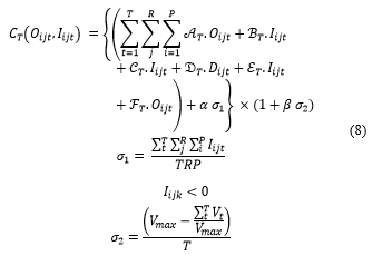Also, the average backlogged orders, and the average volume occupied by the inventory are denoted by  and , respectively. In associate with the planning policy in-use, the values of  may vary. For example, if the customer satisfaction rate is %100, which means shortages are not allowed and . Conversely, if a company unable to deliver their promises on time then  can be set according to the safety stock level. Note, in both cases, the inventory capacity cannot be exceeded, thus . So, a solution candidate is regarded feasible if both conditions are satisfied.

4. Granularity

In systems engineering literature, granularity translates into the level of detail one can decide to consider in a model or decision-making process where the same functionality is expressed with different ‘sized’ designs [30]. In SN, the size of the problem determines the granularity level of the problem which has a significant influence on the computation time and the algorithm’s efficiency. Measures such as the number of product families, the number of facilities, planning periods, etc. are some important factors which affect the granularity level [31]. In this study, in order to verify the robustness of the proposed methodology, three case studies with different granularity levels are considered for the design of experiments represented by a tree structure with two levels and  (Figure 2). The leaves at  denoted by , correspond to an individual scenario with a distinct problem size, known as Small, Medium and Large-scale problems.  is developed based on the problem size categories proposed by Mousavi, Bahreininejad, Musa and Yusof [15], shown in Table 3. The roots at are the number of experiments considered for each category. This is determined according to the number of parameters and the levels of variation of a specific parameter which will be developed using Taguchi method  (see Section 6).

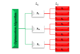Figure 2  Hierarchical structure proposed for implementation phase

• Sizes of the proposed instances [15]

Problem Size	Product Family ( )		Manufacturing Plants ( )	Retailer ( )	Periods ( )
Small	[1-5]	[1-5]		[5-10]	[1-3]
Medium	[6-10]	[1-10]		[11-20]	[1-5]
Large	[11-15]	[11-15]		[20-30]	[6-10]

Note: a problem with  and  is counted as a Medium-scale problem.

5. Solution Approach

To solve the MPMPCSN problem discussed in this paper, GA optimization method is used. GA are based on principles of natural selection and genetics to evolve better solutions through multiple consecutive generations. Selection, Crossover and Mutation are implementations in GA of similar phenomena occurring in the natural world. [23]. Based on the quality of solutions, they have a probability to be selected and evolve in new generations and converge towards optimality. Finally, the solutions are tested against termination criteria (evolving procedure). A good search space and genetic operators must maintain an equilibrium between exploration and exploitation and this is key in reaching optimality [32-34]

5.1.  Generation and Initialization

The first step in implementing the GA is to generate a random population of solutions (chromosomes). Chromosomes are resizable according to problem’s attributes and vary based on the problem type, level of complexity, number and type of variables, granularity, etc. Each chromosome consists of several atomic structures – genes representing the characteristics of the solution  (e.g. number of suppliers, position of manufacturing plants, types of products considered, etc.) [35]. Real coding has been used for this type of problem (Figure 3).

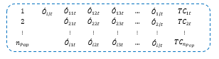Figure 3  Chromosome representation

The performance of the GA is affected by two opposing factors; population size and computation time. The larger the population size; the longer takes the computation time. The population size should be large enough to incorporate sufficient variation in one generation from which the children in the next generations are produced. GA is designed to evolve over a number of generations. Hence, having a large population has a serious impact on the computation time. A carefully selected population size that offers sufficient variety but does permit a fast-enough evolution is needed.

5.2.  Genetic Operators: Selection, Crossover, and Mutation

Genetic operators may affect the optimal fitness value for the designed algorithm. The GA operators presented in this paper are selection, crossover and mutation. Roulette Wheel, Tournament and Ranked are the most popular selection mechanisms that are used in this study [33, 36].

In the following step, the offspring population is created by applying single point crossover and mutation. So, new offsprings are produced by combining the characteristics of two parents that can be better than both parents if they take the best characteristics from each of the parents. This mechanism should be performed with a certain probability. Throughout this study,  and  are referring to crossover and mutation probabilities respectively. Two individuals are produced per randomly selected parents followed by mutating gens of offspring population with specified probability. The mutation is implemented to preserve the variety of the solution pool and prevent GA getting stuck in local optima by exploring the entire search space and maintaining diversity in the population [37]. It is likely that some randomly lost genetic information recovered through mutation. P_m should be set carefully too as such the diversity in the population is preserved but does not negatively affect the overall, fitness of the current population by removing good solutions. Mutation can finely tune the balance between exploration and exploitation. Typically, the mutation rate is small (<2-5%).

5.3.  Simulation

After initializing the first population, each chromosome is evaluated for fitness. Fitness function is a metric used to measure the quality of the represented solution. The fitness value of a chromosome is the most important factor in GA evaluation that is always problem dependent [38]. The fitness function defined for MPMPCSN is the minimum cost of running the network. So the lower the fitness value, the higher is the survival chance of a chromosome.

5.4.  Stopping Conditions

The optimal/near optimal solution is achieved through an iterative procedure until the stopping condition is satisfied. Choosing the termination criteria depends on the complexity of the problem structure as well as the size of the solution pool [39]. Often, the maximum number of generation is adopted which is the case in this study.

The traditional GA has several shortcomings. As a result of premature convergence, the search parameters (selection, crossover, mutation) may not be very useful towards the end of a search procedure [40]. Also, obtaining an absolute global optimum is not guaranteed, however providing good solutions within a reasonable time is generally expected [41, 42]. Also, GA may not be effective if the starting point in search space was at a great distance from optimal solutions [43]. This deficiency limits the use of GA in real-time applications. However, it can be overcome if GA is hybridized with other local search methods where a closed-form expression of the objective function can be appropriately performed [42]. Simulation tools are unique methods that are tightly integrated with mathematical and algorithmic based models. Overall, to improve GA performance and obtain accurate solutions, the population size, selection mechanism, crossover and mutation rates and the computational time are required to be turned. Further validation and evaluation of the proposed model and the solution approach is discussed in the following section.

6. Computational Experiments

This section provides experimental results obtained from applying the proposed SOA methodology on practical tests associated to MPMPCSN problems with different granularity levels.

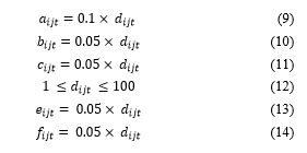
A manufacturing CSN with a central distribution center is considered in which orders received from consumers are being processed. The demand quantities for ,  and  were randomly generated first and remained unchanged throughout the rest of the optimization algorithm (see. Appendix A, Table 22-Table 24), because the variation of  causes changes of other parameters. Also, associated purchase cost per unit of product family  and the corresponding volume  for ,  and are given in Appendix A (Table 21). All other related costs of running the network consist of ordering cost, backordering cost, holding cost, handling cost and transportation cost are computed via (9)-(14). In addition, the fixed parameters of the model are presented in Table 4.

• fixed parameters of the model

Parameters	P	R	T
Small-Scale	5	2	2	1000
Medium-Scale	6	11	5	10000
Large-Scale	10	25	8	100000

Note: P, R, and T are referred to the Product family, Retailer and Planning period respectively.

7. Results and Discussion

As discussed above, the performance of the GA optimization algorithm is mostly influenced by its controllable parameters. These parameters are selection method ( ), crossover and mutation rate ( ), population size ( ) and the maximum number of iteration ( ). Thus, though utilizing Taguchi Orthogonal Array Design along with Regression Analysis and Optimization Solver the optimal parameter set was determined. More details are given in the following sections.

7.1.  Process of Experiment Design

The main two components of the Taguchi method are the number of parameters and their variation levels. In order to analyze the results obtained from ANOVA (analysis of variance) and S/N ratio (signal to noise), it is required to create a set of tables of numbers known as orthogonal arrays. These tables are then used first to reduce the number of experiments, next to determine the most critical parameters with high impact on the outcomes. In this study, we consider the GA controllable parameters as significant factors in 3 levels (Table 7). The Taguchi Orthogonal Array Design ( ) shown in Table 6 is proposed and created by Minitab.

• The parameters’ level

Granularity Level	Small-scale	Medium-Scale	Large-Scale
Parameters	Level 1	Level 2	Level 3
	0.9	0.85	0.8
		0.05	0.025
	[30 60 120]	[100 150 200]	[100 200 300]
	[200 100 50]	[500 400 300]	[3500 3000 2000]

,  and  referred to Roulette Wheel, Tournament and Ranked Selection method respectively

• The layout of the orthogonal array for 5 factors in 3 levels

No.
S1	1	1	1	1	1
S2	1	1	1	1	2
S3	1	1	1	1	3
S4	1	2	2	2	1
S5	1	2	2	2	2
S6	1	2	2	2	3
S7	1	3	3	3	1
S8	1	3	3	3	2
S9	1	3	3	3	3
S10	2	1	2	3	1
S11	2	1	2	3	2
S12	2	1	2	3	3
S13	2	2	3	1	1
S14	2	2	3	1	2
S15	2	2	3	1	3
S16	2	3	1	2	1
S17	2	3	1	2	2
S18	2	3	1	2	3
S19	3	1	3	2	1
S20	3	1	3	2	2
S21	3	1	3	2	3
S22	3	2	1	3	1
S23	3	2	1	3	2
S24	3	2	1	3	3
S25	3	3	2	1	1
S26	3	3	2	1	2
S27	3	3	2	1	3

7.2.  Signal-to-Noise (S/N) Ratio Method

S/N ratios evaluate the size of the apparent effect (signal) against the size of random fluctuations (noise) witnessed in the data. The higher this indicator, the better the compromise is which can be calculated in different ways according to the optimization problem (minimization/maximization) [44]. In this study, S/N ratio values are calculated to determine the best combination of GA control factors. The proposed optimization algorithm was run four times for each parameter set to obtain more refined solutions. The numerical results for the Small, Medium and Large-scale problem are reported in Table 7, Table 8 and Table 9, respectively.

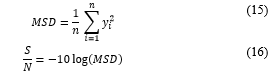
This problem is aimed to minimize the response value (y). Therefore, to minimize the mean-square deviation (MSD) from the target value 0 and maximize the S/N ratio, MSD has to be calculated using (15). The signal to noise (S/N) ratio, in this case, is defined by (16), where  is the sample size.

• Taguchi experimental design and design data of for small-scale problem

Trial No.	Function Evaluation (TC)
	Run 1	Run 2	Run 3	Run 4
1	52545.31	52838.97	52824.62	52798.99	52751.97	138.76	RW	0.9	0.1	30	200
2	57736.13	57984.64	54800.67	56440.22	56740.41	1459.71	RW	0.9	0.1	30	100
3	55082.79	54767.13	55334.41	55983.30	55291.91	516.06	RW	0.9	0.1	30	50
4	57348.28	56895.83	58086.99	58118.95	57612.51	595.84	RW	0.85	0.05	60	200
5	59594.91	58612.27	61314.77	61253.54	60193.87	1321.56	RW	0.85	0.05	60	100
6	60380.16	62646.26	60710.87	59366.54	60775.96	1371.79	RW	0.85	0.05	60	50
7	55536.78	54608.65	55060.74	54506.04	54928.05	471.97	RW	0.8	0.025	120	200
8	55135.85	54540.19	54946.94	56517.07	55285.01	858.15	RW	0.8	0.025	120	100
9	57518.01	59179.99	56537.55	57925.29	57790.21	1094.37	RW	0.8	0.025	120	50
10	52410.97	52718.79	52428.90	52416.20	52493.72	150.24	T	0.9	0.05	120	200
11	53368.53	52881.84	53767.00	52857.57	53218.73	434.73	T	0.9	0.05	120	100
12	58698.26	55432.41	56344.90	57940.46	57104.01	1484.56	T	0.9	0.05	120	50
13	54263.36	56283.66	55064.54	55837.51	55362.27	889.02	T	0.85	0.025	30	200
14	56139.17	56388.68	57656.13	56204.80	56597.20	713.81	T	0.85	0.025	30	100
15	62448.49	94741.69	60631.15	98432.34	79063.42	20304.09	T	0.85	0.025	30	50
16	52413.82	52417.87	52439.46	52418.27	52422.36	11.58	T	0.8	0.1	60	200
17	53546.80	54432.52	53665.56	52804.39	53612.32	666.48	T	0.8	0.1	60	100
18	62686.18	56408.68	56602.45	56552.31	58062.41	3083.61	T	0.8	0.1	60	50
19	54034.56	53650.51	53214.02	53760.76	53664.96	341.24	R	0.9	0.025	60	200
20	56947.05	58519.69	57332.37	56946.45	57436.39	744.73	R	0.9	0.025	60	100
21	62368.65	58889.81	64213.45	64114.90	62396.70	2486.75	R	0.9	0.025	60	50
22	52472.93	52454.69	52466.57	52462.89	52464.27	7.61	R	0.85	0.1	120	200
23	54151.02	54381.73	54913.21	54443.82	54472.45	319.71	R	0.85	0.1	120	100
24	59054.53	58677.67	59390.45	59848.09	59242.69	497.66	R	0.85	0.1	120	50
25	54123.74	53139.69	53600.31	53588.71	53613.11	402.34	R	0.8	0.05	30	200
26	62582.39	57133.15	57636.73	58226.32	58894.65	2498.75	R	0.8	0.05	30	100
27	76782.74	63219.40	67855.77	65419.86	68319.44	5951.48	R	0.8	0.05	30	50

• Taguchi experimental design and design data of for medium-scale problem

Trial No.	Function Evaluation (TC)
	Run 1	Run 2	Run 3	Run 4
1	3055303	3053526	3046047	3050184	3051265.00	4074.87	RW	0.9	0.1	200	500
2	3149794	3154852	3180213	3164676	3162383.75	13396.09	RW	0.9	0.1	200	400
3	3372901	3350114	3335613	3323874	3345625.50	21114.59	RW	0.9	0.1	200	300
4	3200575	3185842	3197118	3191536	3193767.75	6464.29	RW	0.85	0.05	150	500
5	3355893	3308538	3369709	3382514	3354163.50	32301.14	RW	0.85	0.05	150	400
6	3499418	3511169	3529597	3529401	3517396.25	14775.75	RW	0.85	0.05	150	300
7	3432256	3440475	3410509	3433997	3429309.25	13022.82	RW	0.8	0.025	100	500
8	3575145	3520148	3586398	3537586	3554819.25	31141.79	RW	0.8	0.025	100	400
9	4555883	4146796	3846552	4203898	4188282.25	290903.67	RW	0.8	0.025	100	300
10	3051447	3066724	3034552	3045986	3049677.25	13368.15	T	0.9	0.05	100	500
11	3156857	3217344	3129544	3179152	3170724.25	37114.87	T	0.9	0.05	100	400
12	3281164	3310920	3406627	3340245	3334739.00	53652.67	T	0.9	0.05	100	300
13	3077422	3072374	3047223	3078703	3068930.50	14727.31	T	0.85	0.025	200	500
14	3182456	3188477	3166677	3221685	3189823.75	23144.54	T	0.85	0.025	200	400
15	3436084	3441521	3417875	3435688	3432792.00	10294.60	T	0.85	0.025	200	300
16	2991777	2972519	2986549	2982617	2983365.50	8146.47	T	0.8	0.1	150	500
17	3057430	3030744	3064818	3033992	3046746.00	16926.05	T	0.8	0.1	150	400
18	3172227	3184862	3188181	3173263	3179633.25	8079.53	T	0.8	0.1	150	300
19	3360788	3373308	3403272	3440016	3394346.00	35280.59	R	0.9	0.025	150	500
20	3503662	3492818	3501245	3457735	3488865.00	21267.49	R	0.9	0.025	150	400
21	6083231	6707308	6357912	5970323	6279693.50	328268.14	R	0.9	0.025	150	300
22	3099402	3117656	3130297	3111689	3114761.00	12846.33	R	0.85	0.1	100	500
23	3243754	3249067	3272814	3255208	3255210.75	12634.31	R	0.85	0.1	100	400
24	3410574	3462829	3421737	3409948	3426272.00	24965.85	R	0.85	0.1	100	300
25	3232477	3281042	3288839	3245727	3262021.25	27198.93	R	0.8	0.05	200	500
26	3372780	3354390	3375793	3360978	3365985.25	10031.33	R	0.8	0.05	200	400
27	3542951	3526380	3567064	3540808	3544300.75	16865.55	R	0.8	0.05	200	300

• Taguchi experimental design and design data of for large-scale problem

Trial No.	Function Evaluation (TC)
	Run 1	Run 2	Run 3	Run 4
1	6197853	6182641	6205040	6171968	6189375	14895.51	RW	0.9	0.1	100	3500
2	6171968	6197853	6182641	6205040	6189375	14895.51	RW	0.9	0.1	100	3000
3	6026883	6036349	6064389	6092117	6054934	29462.9	RW	0.9	0.1	100	2000
4	6171329	6156044	6162801	6148266	6159610	9813.874	RW	0.85	0.05	200	3500
5	6189910	6160183	6168566	6183770	6175607	13646.61	RW	0.85	0.05	200	3000
6	6276588	6197853	6256788	6232034	6240816	33949.63	RW	0.85	0.05	200	2000
7	5609430	5583614	5604952	5587145	5596285	12806.33	RW	0.8	0.025	300	3500
8	6219773	6220941	6220798	6296291	6239450	37896.94	RW	0.8	0.025	300	3000
9	6393839	6421235	6397965	6500502	6428385	49567.4	RW	0.8	0.025	300	2000
10	5765313	5783485	5797242	5786545	5783146	13270.95	T	0.9	0.05	300	3500
11	6145198	6115210	6141100	6146131	6136910	14630.8	T	0.9	0.05	300	3000
12	6181667	6166755	6174604	6150186	6168303	13526.68	T	0.9	0.05	300	2000
13	5766122	5797580	5768570	5819409	5787920	25393.04	T	0.85	0.025	100	3500
14	6330538	6295429	6350012	6405480	6345365	46003.23	T	0.85	0.025	100	3000
15	6421425	6446814	6429805	6425072	6430779	11227.04	T	0.85	0.025	100	2000
16	6124129	6234488	6150018	6149727	6164591	48152.91	T	0.8	0.1	200	3500
17	6132648	6141044	6166400	6151393	6147871	14537.94	T	0.8	0.1	200	3000
18	5803931	5783648	5803967	5805327	5799218	10400.52	T	0.8	0.1	200	2000
19	5930494	5953702	5898563	5878441	5915300	33387.83	R	0.9	0.025	200	3500
20	6231820	6227294	6232032	6276543	6241922	23183.89	R	0.9	0.025	200	3000
21	6401559	6416416	6425043	6414352	6414342	9699.475	R	0.9	0.025	200	2000
22	6103190	6123392	6079358	6102566	6102126	17999.54	R	0.85	0.1	300	3500
23	5729010	5873701	5867909	5715137	5796439	86089.04	R	0.85	0.1	300	3000
24	6103190	6123392	6079358	6122019	6106989	20598.34	R	0.85	0.1	300	2000
25	6271088	6235294	6240251	6212358	6239748	24169.66	R	0.8	0.05	100	3500
26	6219361	6297088	6249893	6228781	6248781	34642.66	R	0.8	0.05	100	3000
27	6402903	6433575	6407674	6422437	6416647	14017.7	R	0.8	0.05	100	2000

The example of the calculation of S/N ratio for the control parameter  is shown below (column 1 of Table 10) and the results correspond to each case study are summarised in Table 10, Table 11 and Table 12. The difference between the levels of factors in the Table 10- Table 12 determines which parameter has more effect on the quality characteristics (the total cost of the network).

As it can be seen from Table 10, the control factor , by far is the most important factor that impacts on S/N ratio (1.19), ,  and  are also significant factors. Table 11 shows ,  and  are approximately double of  and . Also, in Table 12 while control factor  has a negligible effect in influencing the S/N ratio in  problem, the contribution of all other four parameters (  and ) to the S/N is more than 10%.

The S/N ratios computed for the data set  and  (Table 10-Table 12) are essential for sketching the S/N ratio response diagrams for ,  and  problems (0). So, a higher S/N ratio is related to a data set with the minimum variation which is considered as the best data set.

• The response table of S/N ratio of Problem

	Selection ( )	Crossover Rate ( )	Mutation Rate ( )	Population Size (	Generation ( )
Level 1	-95.08	-94.90	-94.80	-95.46	-94.63
Level 2	-95.16	-95.46	-95.25	-95.16	-95.00
Level 3	-95.22	-95.10	-95.41	-94.84	-95.83
Difference	0.14	0.56	0.61	0.63	1.19

• The response table of S/N ratio Problem

	Selection ( )	Crossover Rate ( )	Mutation Rate ( )	Population Size (	Generation ( )
Level 1	-130.7	-130.9	-130	-130.3	-130
Level 2	-130	-130.3	-130.4	-130.9	-130.3
Level 3	-131.1	-130.6	-131.3	-130.6	-131.4
Difference	1.1	0.5	1.3	0.6	1.4

• The response table of S/N ratio Problem

	Selection ( )	Crossover Rate ( )	Mutation Rate ( )	Population Size (	Generation ( )
Level 1	-135.8	-135.6	-135.6	-135.9	-135.5
Level 2	-135.7	-135.7	-135.8	-135.8	-135.8
Level 3	-135.8	-135.8	-135.7	-135.6	-135.9
Difference	0.1	0.2	0.2	0.3	0.4

Therefore, the best values associated with  and  corresponding to ,  and  problems are as follows: for , level 1(Roulette Wheel selection), level 1 (90% crossover), level 1 (10% mutation), level 2 (120 chromosomes) and level 1 (200 iterations), respectively; for  level 2 (Tournament selection), level 2 (85% crossover), level 1 (10% mutation), level 1 (200 chromosomes) and level 1 (500 iterations), respectively; For  level 2 (Tournament selection), level 1 (90% crossover), level 1 (10% mutation), level 3 (300 chromosomes) and level 1 (3500 iterations), respectively. This can be observed from S/N ratio response diagrams too (Figure 4). The rows show difference values in Table 10-Table 12 determine the contribution level of each parameter in obtaining lower cost. So, the total cost of running the network, for example for  problem, is mostly affected by the number of generation, mutation rate, the selection method, population size and crossover rates of the GA algorithm. To determine the significant level of these parameters, ANOVA method is utilized for which the data given in Table 7- Table 9 are going to be used again. Results obtained from ANOVA are summarized in Table 13-Table 15.

7.3.  ANOVA Method

From ANOVA, the percentage contribution ratio (PCR) of each parameter can be calculated. PCR indicates the significance of all main factors and their interactions on the output. The calculation is performed by comparing the mean square ( ) against an estimate of the experimental errors at specific confidence levels. The total sum of squared deviations ( ) from the total mean S/N ratio is calculated via (17).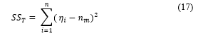

where  is the number of experiments in the orthogonal array and  is the mean S/N ratio for the  experiment.

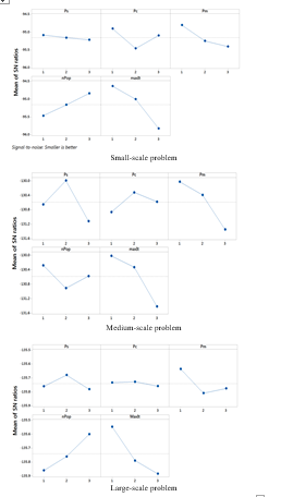Figure 4 The main effect diagram for S/N Ratio response diagram for  parameters ( )

The ANOVA tables for S/N ratios corresponding to the data in Table 10-Table 12 are summarised in Table 13- Table 15. The terms  and  are corresponding to the total sum of squared and the total mean square, respectively. Also, the F-ratios and P-values provided in “F” and “P” columns are calculated via (18) and (19), respectively. F-ratio indicates which parameter ( ) have a significant effect on the quality characteristic ( ) and P-value determines the significant percentage of the parameters on the quality characteristic ( ).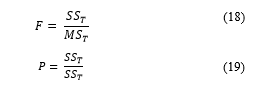

• Results obtained from ANOVA for Small-scale problem

Source
	2	19727169	9863585	0.38	0.685
	2	2.76E+08	1.38E+08	5.32	0.006
	2	3.33E+08	1.66E+08	6.41	0.002
	2	3.49E+08	1.75E+08	6.72	0.002
	2	1.24E+09	6.22E+08	23.96	0
Error	97	2.52E+09	25971697

• Results obtained from ANOVA for medium-scale problem

Source
	2	4.86E+12	2.43E+12	14.27	0
	2	1.69E+12	8.44E+11	4.96	0.009
	2	7.30E+12	3.65E+12	21.45	0
	2	2.07E+12	1.03E+12	6.08	0.003
	2	8.19E+12	4.10E+12	24.08	0
Error	97	1.65E+13	1.70E+11

• Results obtained from ANOVA for large-scale problem

Source
	2	1.02E+11	5.1E+10	1.52	0.223
	2	1.2E+10	5.98E+09	0.18	0.837
	2	3.09E+11	1.55E+11	4.61	0.012
	2	5.93E+11	2.96E+11	8.85	0
	2	1.06E+12	5.30E+11	15.82	0
Error	97	3.25E+12	3.35E+10

Note:  and  stand for the sum of squared and the variance respectively.

It can be observed from Table 13 that the difference between the mean values of the level of the control factor  (selection method) is insignificant (0.68 > 0.05). Therefore, any selection strategy can be chosen for implementation of the proposed SOA for small-scale problem. However, the difference between the mean values of crossover rates ( ), mutation rate ( ) and the number of iteration (Ma ) is significant (0.006, 0.002 and 0.002 < 0.05). Thus, the best control factor setting for maximising the S/N ratio is  at level 1,  at level 1, at level 2 and  at level 1. In the Medium-scale problem, all of the control factors are highly contributing to the performance of the SOA (Table 14). According to Table 15, only  and  are significantly influenced on the performance of the SOA in Large-scale problem, while there is no restriction in choosing the selection strategy and the crossover rate.

7.4.  Confirmation test

The final step of the verification phase is to perform the confirmation test with the optimal level of the GA parameters drawn based on the Taguchi’s design approach for each case study (Table 16).

• The best combination of the parameters

Small-Scale		R	0.9	0.1	120	200
Medium-Scale		T	0.85	0.1	200	500
Large-Scale		R	0.9	0.05	100	3500

The results obtained from the proposed methodology and GA solver associated with ,  and  problems along with the average of the best and the worst results are summarised in Table 17. The quality measurement of the solution is determined according to the value of standard deviation ( ).  Therefore, the solution candidate with the maximum  is considered as the worst solution and the one with the minimum value is regarded as the best solution. Hence, the experiments No. 15 and No. 22 are the worst and the best scenario for the Small-scale problem, respectively.

• The total optimised cost

Problem Size	Small-scale	Medium-scale	Large-scale
Optimal Scenario	49966.28($)	2921429.2($)	5971604 ($)
Best Scenario	52464.27($)	3051265($)	6102126 ($)
Worst Scenario	79063.41($)	6279694($)	6239450 ($)

As can be seen from Figure 5, the proposed algorithm shows better performance compared with the best and the worst solutions acquired from GA solver (5%  ). A similar improvement was also experienced in Medium-scale and the Large-scale problem with 4% and 2% , respectively.

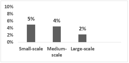Figure 5 Improvement rates obtained from the tuning procedure

Also, the results obtained from the proposed SOA algorithm, and the GA solver associated with , , and  case studies are depicted in Figure 6-Figure 8.

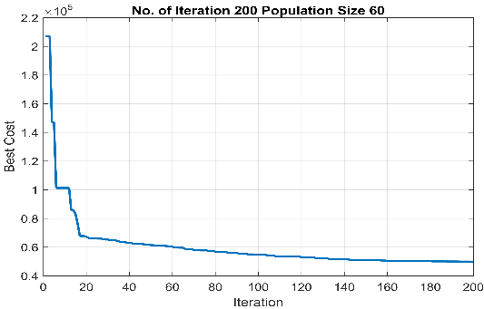
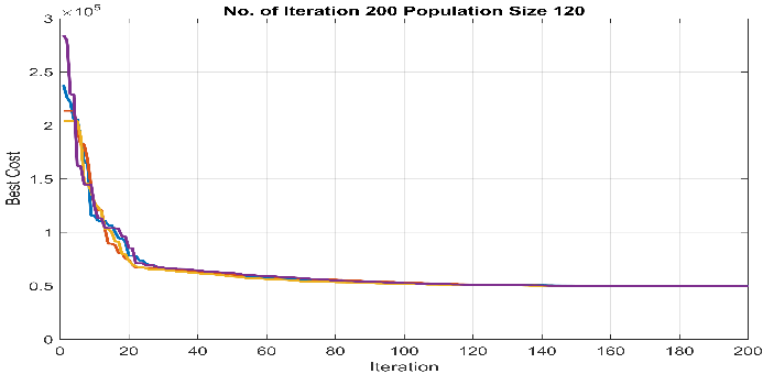
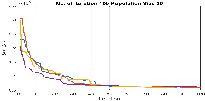Figure 6 Results obtained from (a) the proposed SOA methodology, (b) the GA optimiser ( ) and (c) the GA optimiser ( ) for

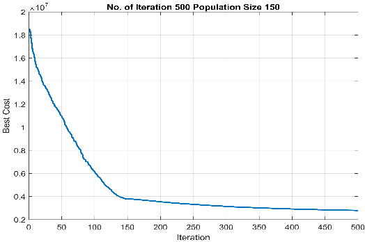
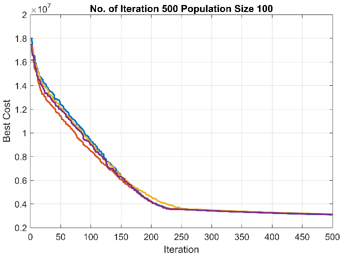
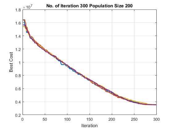Figure 7 Total cost achieved from implementing  (a) the proposed SOA methodology, (b) the GA optimiser () and (c) the GA optimiser () for

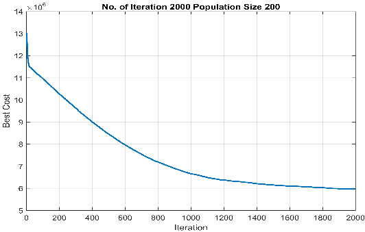
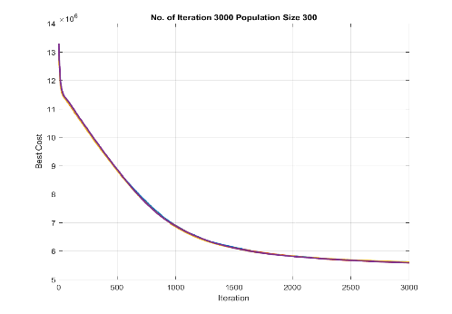
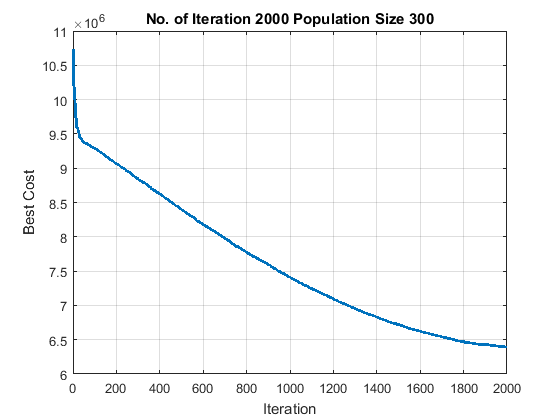Figure 8 Total cost achieved from implementing  (a) the proposed SOA, (b) the GA optimiser ( ) and (c) the GA optimiser ( ) for

Table 18-Table 20 present the optimum quantities associated with each product family to be manufactured for consumers over the given planning horizon.

• The Optimum Solution for Small-scale problem

T1	11	1	54	4	1
T2	10	11	1	5	80
Total	21	12	55	9	81

• The Optimum Solution for Medium-scale problem

T1	136	314	362	220	450	276
T2	391	396	292	575	403	197
T3	369	658	557	574	464	349
T4	499	656	831	433	404	509
T5	577	622	727	681	1013	1086
Total	1972	2646	2769	2483	2734	2417

• The Optimum Solution for large-scale problem

T1	802	706	543	477	471	488	1026	768	670	590
T2	579	480	740	915	561	771	994	820	775	822
T3	710	811	917	608	877	703	952	791	946	1077
T4	1354	1128	630	1161	1058	1222	1090	1099	1427	1187
T5	1507	1771	1624	1429	1524	1229	1145	1537	1254	1554
T6	1685	1935	1762	1952	2055	1802	1848	1903	1397	1698
T7	1997	2192	2097	2037	2118	2435	1883	1918	2276	2854
T8	1904	2411	2159	2765	2271	2542	2309	2604	2437	1998
Total	10252	10371	10455	10606	10575	9608	9815	10685	10187	9990

8. Conclusion and outlook to future

In this paper, an advanced decision-making system for a class of CSN problems was proposed. A novel SOA algorithm incorporating GA as its optimisation module was designed for MPMPCSN problem. The robustness and effectiveness of the proposed methodology was verified through performing twenty-seven computational trials on three practical test problems at different granularity levels (small-scale, medium-scale, large-scale). In addition, a tuning mechanism was recommended to improve the quality of the obtained solutions that was affected by controllable parameters of the optimization module. To this end, two statistical techniques known as ANOVA and Taguchi methods were utilised. The optimum levels associated to the controllable parameters of GA were determined as following: for , level 1(Roulette Wheel selection), level 1 (90% crossover), level 1 (10% mutation), level 2 (120 chromosomes) and level 1 (200 iterations), respectively; for  level 2 (Tournament selection), level 2 (85% crossover), level 1 (10% mutation), level 1 (200 chromosomes) and level 1 (500 iterations), respectively; For  level 2 (Tournament selection), level 1 (90% crossover), level 1 (10% mutation), level 3 (300 chromosomes) and level 1 (3500 iterations), respectively. The proposed SOA was resulted in 5%, 4% and 2% improvement in total cost of CSN associated to , and problems respectively, in contrast to only using GA solver. Also, it was observed that the computational cost and time were reduced significantly.

Conflict of Interest

The authors declare no conflict of interest.

Acknowledgment

The authors are grateful to the Australian Mathematical Society (Aust MS) for providing the Lift-up fellowship which financially supported this work.

1.  Z. Hajiabolhasani, R. Marian, and J. Boland, “Consumer Supply Network Planning: Literature Review And Analysis,” Journal of Multidisciplinary Engineering Science Studies, vol. 3, no. 3, pp. 1519-1538, 2017.
2.  Z. H. Abolhasani, R. Marian, and J. Boland, “Simulation-Optimisation of Multi-Product, Multi- Period Consumer Supply Network using Genetic Algorithms,” in Intelligent Systems Conference (INTELLISYS), London,UK, 2017, pp. 34-44: IEEE, 2017.
3.  X.-S. Yang, S. Koziel, and L. Leifsson, “Computational Optimization, Modelling and Simulation: Past, Present and Future,” in ICCS 2014. 14th International Conference on Computational Science, 2014, vol. 29, pp. 754–758: Procedia Computer Science.
4.  T. Hennies, T. Reggelin, J. Tolujew, and P.-A. Piccut, “Mesoscopic supply chain simulation,” Journal of Computational Science, vol. 5, no. 3, pp. 463-470, 2014.
5.  R. A. Alive, B. Fazlohhahi, B. G. Guirimov, and R. R. Aliev, “Fuzzy-genetic approach to aggregate production–distribution planning in supply chain management,” Information Sciences, vol. 177, pp. 4241-4255, 2007.
6.  N. Mustafee, K. Katsaliaki, and S. J. E. Taylor, “A review of literature in distributed supply chain simulation,” presented at the Simulation Conference (WSC), 2014 Winter, 7-10 Dec. 2014, 2014.
7.  T. M. Pinho, J. P. Coelho, A. P. Moreira, and J. Boaventura-Cunha, “Modelling a biomass supply chain through discrete-event simulation?This work was supported by the FCT – Fundação para a Ciência e Tecnologia through the PhD Studentship SFRH/BD/98032/2013, program POPH – Programa Operacional Potencial Humano and FSE – Fundo Social Europeu,” IFAC-PapersOnLine, vol. 49, no. 2, pp. 84-89, 2016/01/01/ 2016.
8.  F. Campuzano and J. Mula, Supply chain simulation (A system dynamics approach for improving performance). Springer, 2011.
9.  G. Dellino, J. P. C. Kleijnen, and C. Meloni, “Robust optimization in simulation: Taguchi and Response Surface Methodology,” Int. J. Production Economics, vol. 125, pp. 52-59, 2010.
10.  A. Huerta-Barrientos, M. Elizondo-Cortés, and I. F. d. l. Mota, “Analysis of scientific collaboration patterns in the co-authorship network of Simulation–Optimization of supply chains,” Simulation Modelling Practice and Theory, vol. 46, pp. 135-148, 2014.
11.  X. Wan, J. F. Pekny, and G. V. Reklaitis, “Simulation-based optimization with surrogate models—Application to supply chain management,” Computers and Chemical Engineering, vol. 29, pp. 1317–1328, 2005.
12.  J. Y. Jung, G. Blaua, J. F. Pekny, G. V. Reklaitis, and D. Eversdykb, “A simulation based optimization approach to supply chain management under demand uncertainty,” Computers and Chemical Engineering, vol. 28, pp. 2087–2106, 2004.
13.  M. C. Fu, “Optimization via simulation: A review,” Annals of Operations Research vol. 53, pp. 199-247, 1994.
14.  J.-H. Kang and Y.-D. Kim, “Inventory control in a two-level supply chain with risk pooling effect,” International Journal of Production Economics, vol. 135, no. 1, pp. 116-124, 2012.
15.  S. M. Mousavi, A. Bahreininejad, S. N. Musa, and F. Yusof, “A modified particle swarm optimization for solving the integrated location and inventory control problems in a two-echelon supply chain network,” Intell Manuf, 2014.
16.  F. T. S. Chan and A. Prakash, “Inventory management in a lateral collaborative manufacturing supply chain: a simulation study,” International Journal of Production Research, vol. 50, no. 16, p. 15, 15 August 2012 2012.
17.  O. Labarthe, B. Espinasse, A. Ferrarini, and B. Montreuil, “Toward a methodological framework for agent-based modeling and simulation of supply chains in a mass customization context,” Simulation Modelling Practice and Theory, vol. 15, no. 2, pp. 113-136, 2007.
18.  F. Longo and G. Mirabelli, “An advanced supply chain management tool based on modeling and simulation,” Computers & Industrial Engineering, vol. 54, no. 3, pp. 570-588, 2008.
19.  A. Alrabghi and A. Tiwari, “State of the art in simulation-based optimisation for maintenance systems,” Computers & Industrial Engineering, vol. 82, pp. 167-182, 4// 2015.
20.  P. Ghamisi and J. A. Benediktsson, “Feature selection based on hybridization of genetic algorithm and particle swarm optimization,” IEEE Geoscience and Remote Sensing Letters, vol. 12, no. 2, pp. 309-313, 2015.
21.  A. E. Eiben, R. Hinterding, and Z. Michalewicz, “Parameter control in evolutionary algorithms,” IEEE TRANSACTIONS ON EVOLUTIONARY COMPUTATION, vol. 3, no. 2, pp. 124-141, 1999.
22.  J. Sadeghi, S. M. Mousavi, S. T. A. Niaki, and S. Sadeghi, “Optimizing a multi-vendor multi-retailer vendor managed inventory problem: Two tuned meta-heuristic algorithms,” Knowledge-Based Systems, vol. 50, pp. 159-170, 2013.
23.  H. Ding, L. Benyoucef, and X. Xie, “Stochastic multi-objective production-distribution network design using simulation-based optimization,” International Journal of Production Research, vol. 47, no. 2, pp. 479-505, 2009.
24.  A. D. Yimer and K. Demirli, “A genetic approach to two-phase optimization of dynamic supply chain scheduling,” Computers & Industrial Engineering, vol. 58, no. 3, pp. 411-422, 4// 2010.
25.  A. Nikolopoulou and M. G. Ierapetritou, “Hybrid simulation based optimization approach for supply chain management,” Computers & Chemical Engineering, vol. 47, pp. 183-193, 12/20/ 2012.
26.  M. Seifbarghy, M. M. Kalani, and M. Hemmati, “A discrete particle swarm optimization algorithm with local search for a production-based two-echelon single-vendor multiple-buyer supply chain,” Journal of Industrial Engineering International, journal article vol. 12, no. 1, pp. 29-43, 2016.
27.  E. M. Frazzon, A. Albrecht, M. Pires, E. Israel, M. Kück, and M. Freitag, “Hybrid approach for the integrated scheduling of production and transport processes along supply chains,” International Journal of Production Research, vol. 56, 2018.
28.  J. Huang and J. Song, “Optimal inventory control with sequential online auction in agriculture supply chain: an agentbased simulation optimisation approach,” International Journal of Production Research, vol. 56, no. 6.
29.  S. K. Shukla, M. K. Tiwari, H.-D. Wan, and R. Shankar, “Optimization of the supply chain network: Simulation, Taguchi, and psychoclonal algorithm embedded approach,” Computers & Industrial Engineering, vol. 58, no. 1, pp. 29-39, 2// 2010.
30.  B. Unhelkar, Practical object oriented design. Thomson Social Science Press, 2005.
31.  J. Arthur F. Veinott, “Lectures in Supply-Chain Optimization,” S. U. Department of Management Science and Engineering, Ed., ed. Stanford, California, 2005.
32.  B. Fahimnia, L. Luong, and R. Marian, “Genetic algorithm optimisation of an integrated aggregate production–distribution plan in supply chainsn,” International Journal of Production Research, vol. 50, no. 1, pp. 81-96.
33.  D. E. Goldberg, Genetic Algorithms in Search, Optimization, and Machine Learning. MA: Addison-Wesley, 1989.
34.  N. M. Razali and J. Geraghty, “Genetic Algorithm Performance with Different Selection Strategies in Solving TSP,” presented at the Proceedings of the World Congress on Engineering 2011 Vol II, London, U.K., 2011.
35.  B. Fahimnia, “An Integrated Methodology for the Optimisation of Aggregate Production-Distribution Plan in Supply Chains,” Doctor of Philosophy, Mechanical and Manufacturing Engineering, University of South Australia, 2010.
36.  R. Marian, L. Luong, and K. Abhary, “Assembly sequence planning and optimisation using genetic algorithms: part I. Automatic generation of feasible assembly sequences,” Applied Soft Computing vol. 2, no. 3, pp. 223-253.
37.  J.-F. Cordeau, M. Gendreau, A. Hertz, G. Laporte, and J.-S. Sormany, “New heuristics for the vehicle routing problem,” in Logistic Systems: Desing and Optimization, A. Langevin and D. Riopel, Eds. United States of America: Springer, 2005, pp. 279-298.
38.  R. M. MARIAN, “Optimisation of assembly sequences using genetic algorithms,” DOCTOR OF PHILOSOPHY, School of Advanced Manufacturing and Mechanical Engineering, UNIVERSITY OF SOUTH AUSTRALIA, 2003.
39.  F. T. Chan, S. Chung, and S. Wadhwa, “A hybrid genetic algorithm for production and distribution,” Omega, vol. 33, no. 4, pp. 345-355, 2005.
40.  Z. H. Abolhasani, R. M. Marian, and L. Luong, “Optimization of Multi-Commodities Consumer Supply Chain- Part 1- Modelling,” Journal of Computer Science, vol. 9, no. 12, p. 16, 2013.
41.  H. Xing, X. Liu, X. Jin, L. Bai, and Y. Ji, “A multi-granularity evolution based Quantum Genetic Algorithm for QoS multicast routing problem in WDM networks,” Computer Communications, vol. 32, pp. 386-393, 2009.
42. C. A. C. Coello, G. B. Lamont, and D. A. V. Veldhuizen, D. E. Goldberg and J. R. Koza, Eds. Evolutionary algorithms for solving multi-objective problems, 2nd ed. (Genetic and Evolutionary Computation). New York: Springer, 2007.
43.  Jeong Hee Hong, K.-M. Seo, and T. G. Kim, “Simulation-based optimization for design parameter exploration in hybrid system: a defense system example,” Simulation: Transactions of the Society for Modeling and Simulation International, vol. 89, no. 3, pp. 362-380, 2013.
44.  P. Genin, S. Lamouri, and A. Thomas, “Multi-facilities tactical planning robustness with experimental design,” Production Planning & Control, vol. 19, no. 2, pp. 171-182, 2008/03/01 2008.

(Click Here)

(Click Here)