1. Introduction

This paper is continuation for our work presented in [1]. DC motors are applied in one way or the other in factories, home appliances, computers to robots, airplanes, and cars. They are more widely used than the related machines, the AC motors, owing to their diverse favorable characteristics. These characteristics some of which are, linear speed control properties and high starting torque. There are more than one types DC motors and all these types have numerous benefits over AC motors which include: less heat production, simpler controllers used, have higher efficiency, can offer precise position control, can produce very close to constant torque and they are easily controllable [2-11]. For that reason, the adoption of DC motors will reduce the amount of energy consumed and improve the efficiency of the machines they are installed. The improvement of DC motors’ control arrangement to enhance their response characteristics is one way of achieving these. Is so doing, they will be able to accomplish their work efficiently without the necessarily increasing the capacities of motors alongside their control circuits [12-16].

Researchers have previously done a lot of work to design DC motor control circuits with or without the use of Kalman Filter (KF) and/or Fuzzy Logic Controller (FLC). In [2] the researchers introduced a feedback and feedforward system controllers to control DC motor. While the feedforward loop was just a gain represented by , the feedback loop was PD controller with gains denoted by  and . The gains were optimized using fuzzy logic and genetic algorithm and all were constant. A PC was used in [3] to implement a DC motor PID controller, it was configured by trial and error to attain the desired performance. This study also applied a photo sensor to estimate the motor speed and transmit it to the personal computer. In [17] the researchers came up with a torque estimator for DC motors by means of adaptive Kalman filter consisting of two sections; estimation and extraction. Each of these parts is a DC motor’s mathematical model and the first one had one more PID controller to guarantee the accuracy of the estimation. Although it required current and speed sensors, this estimator was designed with no torque sensors. A state feedback controller was developed by the researchers in [4] with the use of Extended Kalman Filter (EKF) for induction motor and KF for DC motor to evaluate the states. A DC motor was controlled using a PID controller in [5],      were dynamically modified online by three distinct FLC controllers, one for each gain. KF was utilized for tuning the Membership Functions (MFs) of such FLCs. The FLC controllers, in [7,10], were intended to control DC motors. Microcontrollers was used to implement both FLCs and both made use physical sensors ,that is, no estimators were introduced in these studies. In [9], the researchers made use of a Kalman filter,  torque sensor and current sensor to measure the speed of a DC motor and thereafter fed it back to a PI controller to enhance the motor’s speed estimation. In [11], the DC motor speed was estimated using Kalman filter and was controlled using both Linear–Quadratic Regulator (LQR) and PID controllers. In [18], the authors adjusted the widths of FLC membership functions by means of arithmetic averaging technique and feed forward to run the DC motor without the use of feedback to minimize online computational needs.

The objective of this study is to realize better transient and steady-state responses for a DC motor’s speed control (separately excited brushed type) and efficient reference speed tracking irrespective of load and alteration of reference speed. The voltage will only be used as the output of the controller, while the current will not be controlled but restricted within the rated motor current. Then the results from the PID controller and conventional PID controller will be compared with the PID-type FLC controller (FLC-PID) and KF. In addition to the classical time response characteristics; the performance index of IAE is selected to illustrate the achievement in the motor speed response. IAE displays the total error for the entire run period of the simulation to increase the size of the built controller in tracking command speed, notwithstanding its variations and changes in load. In Section 2 below, the DC motor model is developed, Section 3 covers the KF design, Section 4 addresses the different controller designs, and Section 5 carries the conclusion.

2.  DC Motor Model

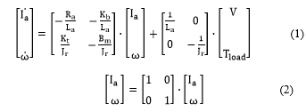
The most common type of DC motors which are broadly applied in robotic and industrial functions is the separately excited DC motor with constant excitation field can be represented by state-space model [4,13]. This model comprises two differential equations representing the mechanical and electrical responses of the DC motor in both static and active operating states. Equations (1) and (2) illustrate this model [4,19].

The chosen motor specification are listed in Table 1 [20].

The values from Table I are substituted in (1) and (2) and a sampling time ( ) of 1 millisecond was chosen. Then, using a MATLAB (c2d) function, the continues state-space equations are changed to discrete. The discrete-time state-space motor model is shown in (3) and (4):

Where (t) represents the current sample, and (t+1) denote the next sample.

3. Kalman Filter Observer

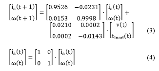
As mentioned in [21,22]  Kalman filter is considered as optimum observer for the state variables and the outputs of linear time-invariant (LTI) systems. It has two significant characteristics which made it our choice to estimate the states of the DC motor under study; one it is able to exploit the already known state-space model of the DC motor, and the second reason because it has the capacity to filter diverse sensor noises [23]. The Kalman filter system discrete equations can be broken into two categories and are illustrated in (5)-(10) [23].

A.    Time update equations

B.    Measurement update equations

In which  is the estimated current state vector;  is the estimated process error covariance matrix;  is the estimated noise matrix;  is the system noise covariance matrix;  is Kalman gain; : is the transformation matrix;  is sensor noise covariance matrix;  is measurement of the state;  is Kalman filter  matrix for state-space model of the system under study (in this case the DC motor);  is the measured states vector;  is measurement noise;  is corrected state vector; and,  is corrected process error covariance matrix

Kalman filter estimates the states of present system and the error in such estimates by means of the time update equations. It then rectifies these errors using the measurement update calculations based on the Kalman gain and the actual inaccurate measurement. This done in a repetitive way for all sample times ( ) or time steps [23]. Let  and  represent the error in speed and current calculation/measurement correspondingly.

 Then accurate  computation needs the integration of  and  as illustrated in (11), which is solving the second row of (1) for :

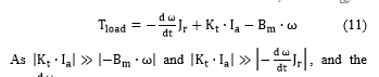As  and , and the term  has noise because of the differentiation, The approximate formula below can be used to solve :

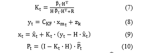
Equation (13) is derived by solving the first row of (3) for ω, is used to calculate the motor speed:

Because ,  can be calculated with high enough accuracy using (14) below:

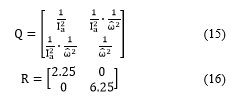
The sensors and process noise covariance matrices are articulated in terms of the stochastic characteristics of their respective noises and they can be either static or dynamic [24]. Q elements were found to be directly proportional to the inverse of the estimated armature current and motor speed and therefore was chosen to be dynamic as shown in (15). Since the sensor error is fixed by the manufacturer in its datasheet, R was selected to be static. In (16) the calculations of R are shown and the datasheet of a sample current sensor is found in [25].

4. Controller Design, Simulation and Results

In this section, three potential designs of a controller for DC motor speed control are discussed. Figure 1 shows the general system architecture under study.

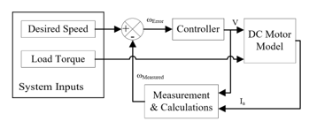Figure 1: The DC motor with the PID controller and speed feedback

4.1.  Discrete PID Controller

Initially, discrete PID was used to control the DC motor. The transfer function of the controller is presented in (17). Figure 2 shows the command speed signal to the motor, the motor will experience an uncontrolled torque load variation illustrated in Figure 3. In the rest of this work, Figure 2 and Figure 3 will be considered as the running conditions for the DC motor under study.

Using MATLAB/Simulink PID tuner with “design focus” option set to “Reference tracking”, a discrete PID controller was tuned to control the motor’s speed by means of changing its supply voltage. The gains after MATLAB/Simulink PID tuner are: =2.51, =9.724, =-0.19185 and N=12.89.

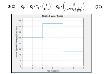Figure 2 Desired motor speed profile

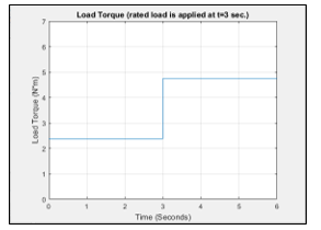Figure 3 Load torque (disturbance) profile

To simulate current and voltage sensors precision tolerances, arbitrary noise of 2% was added to voltage and current [25]. The voltage (controller output) was kept at or below the nameplate voltage that is 220 V, and this limitation is kept for the FLC PID in part C and throughout this work. The measurement of current was restricted certain upper limit to mimic the current sensor magnetic limitation characteristics. In the measurement block, the speed is determined using (13) only and no more conditioning is required. Figure 4 demonstrate the system response in which the system experienced an IAE of 47.52, settling time ( ) of 1.08 second and peak overshoot of 25.7%. Using (14) to obtain ω in the subsequent run lowered the peak overshoot to 23.7% and lowered the IAE a little making it 45.89. The settling time experienced a slight fall to 1.07 seconds. Such a small enhancement in system response is associated to the cancelation of the noisy derivative section in (13). The measured and actual motor speed using (13) and with no Kalman filter are displayed in Figure 5.

4.2.  PID with KF

Kalman filter was applied in the next run in an effort to predict the motor’s speed, Figure 6 shows the whole system. When Kalman filter was used and everything else as from the previous run was unchanged, Figure 7 displays clear falls in the settling time, IAE and peak overshoot which are now in order, 0.635, 36.71 and 8.01%. The KF estimated speed of the motor vs the actual and measured speeds are shown in Figure 8.

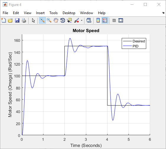Figure 4 motor speed response with PID and unit feedback

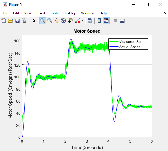Figure 5 actual motor speed and measured motor speed with added noise

Figure 6 The DC motor with the PID controller and Kalman filter

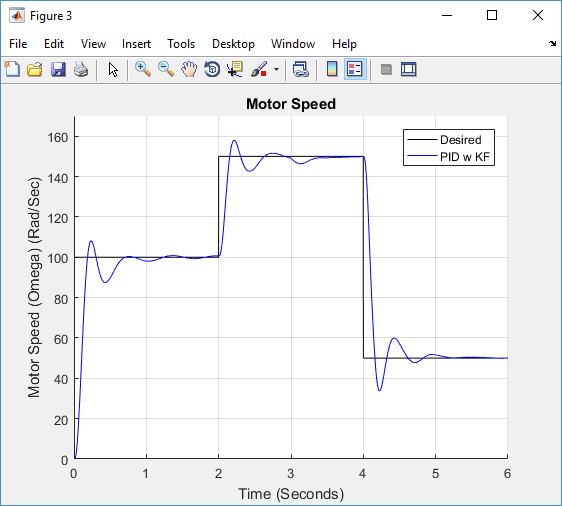Figure 7 motor speed response with PID and Kalman filter estimator

While it showed some improvement in the system response, the PID with the help of Kalman filter was unable to fully remove the overshoot of the motor’s speed response which introduced unwanted ringing in the motor’s speed. This limitation can be overcome by designing a PID-type fuzzy logic controller with PID properties and the additional variable gains throughout the full range of the controller’s operation [26,27].

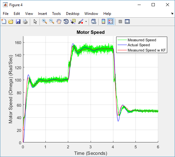Figure 8 actual motor speed and measured motor speed with added noise with and without Kalman filter

4.3.  FLC-PID Controller

A Takagi-Sugeno type FLC-PID controller is chosen in this work as it is “more diverse in gain variation characteristics” than the Mamdani type FLC-PID controller  [26]. Aside from few changes in the rule base; the main difference in design between Takagi-Sugeno type FLC-PID controller developed in this work and the one utilized in [28,29] is the different and distinct gains for PI and PD controllers, offering an additional degree of design freedom. Figure 9 represents the block diagram of the FLC-PID developed for this work.

For both controllers (FLC-PI and FLC-PD), the input and output signal ranges were normalized to [-1,1]. Doing so will enable this FLC-PID controller to be applied for various motor sizes by just tuning its gains. Figure 10 shows the MF’s for error as well as rate of change of error, Gaussian type was chosen to guarantee smooth control action. The MF’s for the controller’s output are presented in Figure 11 which are uni-valued MF’s. one benefit of using FLC controller is that we can make all the equivalent MF’s similar for both FLC-PD and FLC-PI, and the unique action variation between the controllers is achieved only by altering their rule base. Which is what we did in this work.

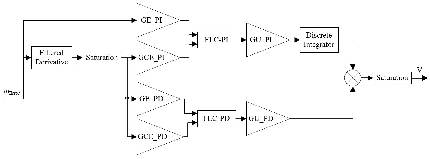Figure 9 FLC-PID block diagram

Where GE_PI is FLC-PD speed error gain; GCE_PI is FLC-PD change of rate of speed error gain; GU_PI is FLC-PD output gain; GE_PD is FLC-PD speed error gain; GCE_PD is FLC-PD change of rate of speed error gain; and, GU_PD is FLC-PD output gain.

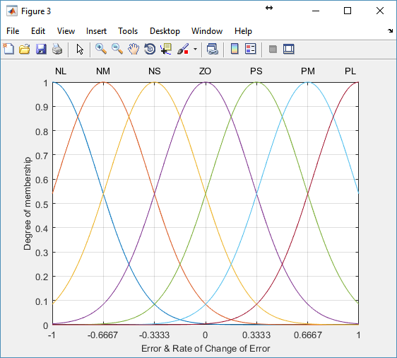Figure 10 input membership functions for FLC-PI and FLC-PD

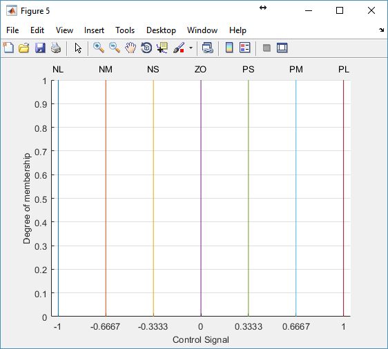Figure 11 output membership functions for FLC-PI and FLC-PD

The rule base for FLC-PD and FLC-PI are shown by Tables 2 and 3 respectively. The FLC-PID applies these rules in the arrangement illustrated in (17) [30]to produce the control surfaces presented in Figure 12 and 13. Such rules simulates the performance of the common PI and PD controllers to develop FLC-PI and FLC-PD controllers in that order.

Table 2 FLC-PD rule base

Control Output UPD		Error (e)
		NL	NM	NS	ZO	PS	PM	PL
Rate of Change of Error (ce)	PL	PS	PS	PM	PL	PL	PL	PL
	PM	PS	PS	PS	PS	PL	PL	PL
	PS	PM	PS	PS	PS	PM	PL	PL
	ZO	NL	NM	PS	ZO	PS	PM	PL
	NS	NL	NL	NM	NS	PS	PS	PM
	NM	NL	NL	NL	NS	PS	PS	PS
	NL	NL	NL	NL	NS	PS	PS	PS

Table 3 FLC-PI rule base

Control Output UPI		Error (e)
		NL	NM	NS	ZO	PS	PM	PL
Rate of Change of Error (ce)	PL	ZO	PS	PL	PL	PL	PL	PL
	PM	NS	ZO	PS	PM	PL	PL	PL
	PS	NL	NS	ZO	PS	PM	PL	PL
	ZO	NL	NM	NS	ZO	PS	PM	PL
	NS	NL	NL	NM	NS	ZO	PS	PL
	NM	NL	NL	NL	NM	NS	ZO	PS
	NL	NL	NL	NL	NL	NL	NS	ZO

Where PL is Positive Large; PM is Positive Medium; PS is Positive Small; ZO is Zero; NS is Negative Small; NM is Negative Medium; and NL is Negative Large.

When we have (17), Tables 2 and 3, Figure 10, 11, 12 and 13 into perspective; it would be obvious that both FLC have more than 49 equations and more than 10 parameters (comprising membership functions parameters) to adapt its output. These add to diverse design flexibility for the preferred control surface that the common PID controller simply cannot provide.

Figure 12 FLC-PD control surface

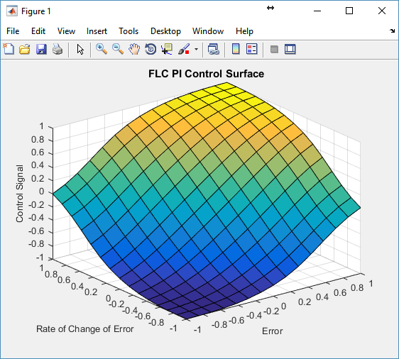Figure 13 FLC-PI control surface

The next five steps briefly describe how an FLC works [30,31,32]:

1. The input signals are mapped to their corresponding MF’s and assign degree of membership ranging between [0,1] for each input signal. (Fuzzification stage)
2. Finding the degree of firing of each rule by applying fuzzy logic operation (e.g. AND, OR, … etc.) to the antecedents. (Inference mechanism matching stage1).
3. FLC determines which rule is to be fired by checking the result from step 2, each rule having a nonzero result will be fired. (Inference mechanism matching stage 2).
4. Multiply the consequent of each rule by its firing degree (the corresponding result from step 3). (Inference setup/aggregation stage).
5. Apply the selected defuzzification method (for this work weighted average method was selected, which is shown in equation 18). (Defuzzification stage).

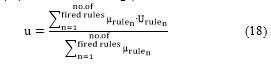where:

: is FLC output

: is the firing degree for each rule (step 2 above)

: is the consequent of .

The selection of FLC-PID gains was informed by the following: because the rated speed of the motor is 157.08 rad/sec, speed error gains were calculated as   . A range of [-1000,1000] was taken for derivative of error to neutralize high values due to the derivative term; consequently, it’s gain was chosen to be . Lastly, the output gains is set to be  to put an accelerated control action to the motor’s speed. FLC-PID gains first estimation may as well be acquired from an adjusted PID as stated in [28].

4.4.  Gains’ Value Optimization Using GA

Genetic algorithm (GA) is an evolutionary algorithm; it uses the process of natural selection to solve optimization problems; it works to find the fittest value in the range of search regardless of that range’s nonlinearity. Simple GA can be summarized in the following steps [33]:

1. Convert the variable values into binary. (Initialization 1)
2. Initiate random population of 50 individual per variable. (Initialization 2)
3. Check the fitness of each individual. (Fitness 1)
4. Select the best-fitted individuals. (Fitness 2)
5. Generate new individuals (children) by combining two individuals (parents) from step 4. (Crossover)
6. Generate new individuals (children) by making random changes to individuals (parents) from step 4. (Mutation)
7. Replace the current population with the children from steps 4 and 5. (Initiate new generation)
8. Repeat from step 3 until at least one stopping condition (number of generations, the value of the relative change in the fitness function, … etc.) is satisfied.

Table 4 tuned controller gains

Gain	Value
GE_PI
GCE_PI
GU_PI
GE_PD
GCE_PD
GU_PD

MATLAB optimization tool with built-in GA optimizer has been used in this project to fine tune the FLC-PID gains. The selected fitness function was the IAE of the speed, to ensure that the tuning is aimed at faster and improved speed command tracking with an all-round load change rejection. Because GA is a stochastic search tool, various runs may produce varying results, but each result must satisfy a minimum of one stopping condition. Indeed, the remaining runs with various gains can result in similar system response. Table 4 shows the FLC-PID gains upon tuning.

The FLC-PID successfully removed the peak overshoot (less than 0.5%), decreased the settling time to 0.257 seconds and reduced the IAE to only 20.1. To make this clearer, Table 4 illustrates a percentage contrast between FLC-PID with KF, common PID without KF and PID with KF, choosing common PID without KF as a 100% base. Figure 14 is a graph of the motor speed response for all scenarios mentioned above versus the desired speed. It is worth noting that lower value for every performance index used in this paper means improved system response.

Figure 14 compare motor speed for all three controllers used in this work

Table 4 comparison of system response for all three controllers used in this work

Performance Indices	PID W/O KF	PID With KF	FLC-PID With KF
Settling time (seconds)	1.07 100%	0.635 59.35%	0.257 24.02%
Peak Overshoot (radians)	23.7 100%	8.01 33.8%	<0.5 <2.11%
IAE	45.89 100%	36.71 80%	20.1 43.8%

4.5.  Converting FLC-PID to lookup Table

In order to reduce the computational requirement of FCL-PID to a real word controller e.g. microcontroller or field programmable gate array (FPGA), thus making it easier for the controller to response in real time, the FLC-PI and FLC-PID control surfaces will be stored in a linear lookup-Table format. This can be done by dividing the two inputs of both FLC controllers (FLC-PI and FLC-PD) into  breakpoints (since both inputs range is normalized to , 21 breakpoints mean 0.1 spacing) and evaluate the FLC controllers at each of the breakpoints. The total evaluations will be  for each FLC controller. A linear interpolation based lookup Table was put in place of each FLC controller in the controller block as shown in Figure 15, and they were loaded with the corresponding 441 evaluations. The motor speed response with FLC-PID and lookup Table FLC-PID are shown in Figure 16. Both responses are actually overlapping as the difference between them is minimal. A zoomed view of the speed response from the time 0.3to 0.7 seconds is shown in Figure 17 to magnify the difference between these responses, which has a maximum value of less than . As a result, the DC motor with the lookup Table had almost identical performance indices (the difference is less than 0.1%) as compared to the response with the actual FLC-PID controller.

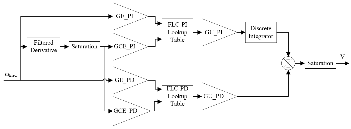Figure 15 lookup table FLC-PID block diagram

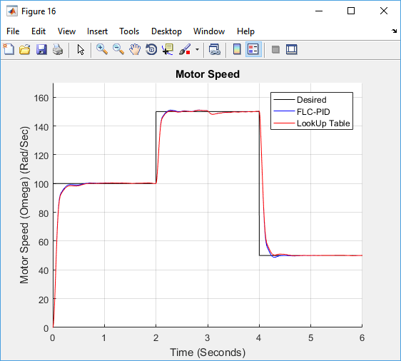Figure 16 lookup table FLC-PID versus actual FLC-PID speed response

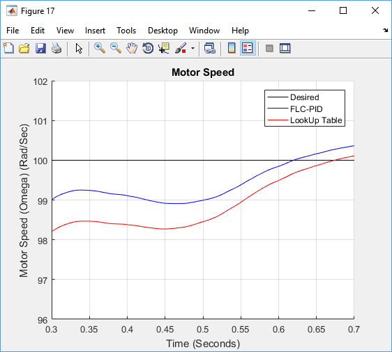Figure 17 zoomed view of lookup Table FLC-PID versus actual FLC-PID speed response

5. Conclusion

This work investigated the sensorless speed control of fixed field DC motor in a noisy environment mimicking real-live operating environment. As a result of noise in this environment, a common PID controller yielded high peak overshoot from the reference and took significate time to settle. That was true even after removing the noisy derivative terms in  and  in their respective estimation equations. When using Kalman filter, the PID controller was able to lower the peak overshoot by good margin, nonetheless it stayed there with long ringing in the speed response. To minimize these undesirable system behaviors , an FLC-PID controller was applied to the motor. This controller was tuned by GA. This new controller design end up reducing the peak overshoot to less than 1% and the settling time by 75.98%. The IAE was also reduced to only 56.2% of what it was. Finally, the FLC-PID was converted into linear interpolation- based lookup-Table to reduce the computational complexity of the FLC-PID and make it easier to realize in real world applications while maintaining the same response as with the actual FLC-PID. Achieving these enhanced time response and speed tracking improvement will ensure smoother, more robust and more power saving operation of the motor. The FLC-PID gave the DC motor “immunity” to reference speed and load changes as long as these changes are within its operating capacity.

In the future we intend to implement the lookup-Table by using a specialized lookup-Table Integrated Circuit (IC) or a generic Field Programmable Gate Array (FPGA) IC and to connect it to a physical separately excited DC motor in an experimental setup. Variable load, variable reference speed and current limiting protection must be included in this setup. This implementation will require retuning the FLC-PID gains, but in return it will solidly verify the proposed controller.

Conflict of Interest

The authors declare no conflict of interest.

1.  A. Y. Al-Maliki and K. Iqbal, “FLC-based PID controller tuning for sensorless speed control of DC motor,” Proc. IEEE Int. Conf. Ind. Technol., vol. 2018–February, pp. 169–174, 2018.
2.  S. Chowdhuri and A. Mukherjee, “An evolutionary approach to optimize speed controller of DC machines,” Proc. IEEE Int. Conf. Ind. Technol. 2000 (IEEE Cat. No.00TH8482), vol. 2, pp. 682–687, 2000.
3.  G. Huang and S. Lee, “PC-based PID speed control in DC motor,” 2008 Int. Conf. Audio, Lang. Image Process., pp. 400–407, 2008.
4.  G. G. and P. Siano, “Sensorless Control of Electric Motors with Kalman Filters: Applications to Robotic and Industrial Systems,” Int. J. Adv. Robot. Syst., vol. 8, no. 6, p. 1, 2011.
5.  M. Shadkam, H. Mojallali, and Y. Bostani, “Speed Control of DC Motor Using Extended Kalman FilterBased Fuzzy PID,” Int. J. Inf. Electron. Eng., vol. 3, no. 9, pp. 1209–1220, 2013.
6.  J. Jacob, S. S. Alex, and A. E. Daniel, “Speed Control of Brushless DC Motor Implementing Extended Kalman Filter,” Int. J. Eng. Innov. Technol., vol. 3, no. 1, pp. 305–309, 2013.
7.  A. A. Thorat, S. Yadav, and S. S. Patil, “Implementation of Fuzzy Logic System for DC Motor Speed Control using Microcontroller,” J. Eng. Res. Appl., vol. 3, no. 2, pp. 950–956, 2013.
8.  J. N. Rai and M. Singhal, “Speed Control of Dc Motor Using Fuzzy Logic Technique,” IOSR J. Electr. Electron. Eng., vol. 3, no. 6, pp. 41–48, 2012.
9.  P. Deshpande and A. Deshpande, “Inferential control of DC motor using Kalman Filter,” in 2012 2nd International Conference on Power, Control and Embedded Systems, 2012, pp. 1–5.
10.  H. R. Jayetileke, W. R. De Mel, and H. U. W. Ratnayake, “Real-time fuzzy logic speed tracking controller for a DC motor using Arduino Due,” 2014 7th Int. Conf. Inf. Autom. Sustain. “Sharpening Futur. with Sustain. Technol. ICIAfS 2014, 2014.
11.  T. Abut, “Modeling and Optimal Control of a DC Motor,” Int. J. Eng. Trends Technol., vol. 32, no. 3, pp. 146–150, Feb. 2016.
12.  A. O. Al-Jazaeri, L. Samaranayake, S. Longo, and D. J. Auger, “Fuzzy Logic Control for energy saving in Autonomous Electric Vehicles,” in 2014 IEEE International Electric Vehicle Conference (IEVC), 2014, pp. 1–6.
13.  A. Watanabe, S. Yuta, and A. Ohya, “A new method for efficient drive and current control of small-sized brushless DC motor: Experiments and its evaluation,” in IECON 2010 – 36th Annual Conference on IEEE Industrial Electronics Society, 2010, pp. 735–741.
14.  L. Varghese and J. T. Kuncheria, “Modelling and design of cost efficient novel digital controller for brushless DC motor drive,” in 2014 Annual International Conference on Emerging Research Areas: Magnetics, Machines and Drives (AICERA/iCMMD), 2014, pp. 1–5.
15.  Y.-P. Yang and M.-T. Peng, “A Surface-Mounted Permanent-Magnet Motor With Sinusoidal Pulsewidth-Modulation-Shaped Magnets,” IEEE Trans. Magn., vol. PP, pp. 1–8, 2018.
16.  S. Noguchi and H. Dohmeki, “Improvement of efficiency and vibration noise characteristics depending on excitation waveform of a brushless DC motor,” 2018 IEEE Int. Magn. Conf., pp. 1–5, 2018.
17.  S. Lee and H. Ahn, “Sensorless torque estimation using adaptive Kalman filter and disturbance estimator,” in Proceedings of 2010 IEEE/ASME International Conference on Mechatronic and Embedded Systems and Applications, 2010, pp. 87–92.
18.  J. K. Satapathy, S. Das, C. J. Harris, and P. Misra, “Indirect tuning of membership function in a fixed fuzzy structure for efficient control of a DC drive system,” in SMC 2000 Conference Proceedings. 2000 IEEE International Conference on Systems, Man and Cybernetics. “Cybernetics Evolving to Systems, Humans, Organizations, and their Complex Interactions” (Cat. No.00CH37166), 2000, vol. 5, pp. 3790–3793.
19.  S. P. Paul C. Krause, Oleg Wasynczuk, Scott D. Sudhoff, Analysis of Electric Machinery and Drive Systems, 3rd ed. Piscataway, NJ, USA: John Wiley & Sons, Inc., 2013.
20. F. Rashidi, M. Rashidi, and A. Hashemi-Hosseini, “Speed regulation of DC motors using intelligent controllers,” Control Appl., pp. 925–930, 2003.
21.  F. L. Lewis, L. Xie, and D. Popa, Optimal and Robust Estimation With an Introduction to Stochastic Control Theory, Second Edi. CRC press, 2008.
22. R. E. Kalman, “A New Approach to Linear Filtering and Prediction Problems,” J. Basic Eng., vol. 82, no. 1, p. 35, 1960.
23.  R. G. Brown and P. Y. C. Hwang, Introduction to Random Signals and Applied Kalman Filtering WITH MATLAB EXERCISES, FOURTH EDI. John Wiley & Sons, Inc., 2012.
24.  Texas Instruments and T. I. Europe, “Sensorless Control with Kalman Filter on TMS320 Fixed-Point DSP,” Control, no. July, 1997.
25.  “Split Core Current Transformer ECS1030-L72.” ECHUN Electronic Co., Ltd, Dongguan City. Guang Dong. China, pp. 1–3, 2017.
26.  H. Ying, “Constructing nonlinear variable gain controllers via the Takagi-Sugeno fuzzy control,” IEEE Trans. Fuzzy Syst., vol. 6, no. 2, pp. 226–234, 1998.
27.  B. M. Mohan and A. Sinha, “Analytical structure and stability analysis of a fuzzy PID controller,” Appl. Soft Comput., vol. 8, no. 1, pp. 749–758, 2008.
28.  A. Noshadi, J. Shi, W. Lee, and A. Kalam, “PID-type fuzzy logic controller for active magnetic bearing system,” in IECON 2014 – 40th Annual Conference of the IEEE Industrial Electronics Society, 2014, vol. 27, no. 7, pp. 241–247.
29.  J. X. Xu, C. C. Hang, and C. Liu, “Parallel structure and tuning of a fuzzy PID controller,” Automatica, vol. 36, no. 5, pp. 673–684, 2000.
30. K. M. Passino and S. Yurkovich, Fuzzy Control. Addison Wesley Longman, Inc., 1998.
31. G. S. Sandhu, T. Brehm, and K. S. Rattan, “Analysis and design of a proportional plus derivative fuzzy logic controller,” in Proceedings of the IEEE 1996 National Aerospace and Electronics Conference NAECON 1996, 1996, vol. 1, pp. 397–404.
32.  S. Z. Hassan, H. Li, T. Kamal, F. Mehmood, “Fuzzy embedded MPPT modeling and control of PV system in a hybrid power system” in 12th International IEEE Conference on Emerging Technologies (ICET) 18-19-October 2016
33.  D. A. Coley, An Introduction to Genetic Algorithms for Scientists and Engineers. WORLD SCIENTIFIC, 1999.

(Click Here)

(Click Here)