1. Introduction

In Robot that autonomously decides action based on surrounding environmental information such as disaster rescue robot and robot cleaner needs to optimize multiple objectives simultaneously, such as moving as fast as possible to the target location, increasing safety, reducing consumption of fuel and batteries, etc. However, in multi-criteria decision making, objectives often conflict with each other, and in such cases there does not exist complete optimal solutions that simultaneously minimize or maximize all the objectives. Instead of a complete optimal solution, a solution concept, called Pareto optimality, is introduced in multi-objective optimization, and many efforts are accumulated to find a set of Pareto optimal solutions [1]. At a Pareto optimal solution, in order to improve a certain objective function, we have to sacrifice one or more other objective functions. Moreover, when there exist two or more Pareto optimal solutions, a decision maker selects the most preferred solution from among the Pareto optimal solution set based on his or her own preference. However, a complex procedure is required to identify the preference structure of the decision maker [2]. If we interpret each Pareto optimal solution as a candidate and try to select one solution out of the Pareto optimal solution set, we do not necessarily need to identify the preference structure of the decision maker. Then, we can employ an interactive decision making method that derives a so-called preference solution of the decision maker by using the local preference information obtained from an interactive process with the decision maker [3-5].

As a solution method for linear or convex optimization problems, it is possible to apply mathematical solution methods finding an exact optimal solution such as the simplex method, the successive quadratic programming, and the generalized reduced gradient method. On the other hand, for non-convex or discontinuous optimization problems, we have to employ some approximate optimization methods such as evolutionary computation methods including genetic algorithm, genetic programming, and evolution strategy. Such evolutionary technologies include swarm intelligence such as particle swarm optimization, ant colony optimization and so on. Effectiveness of such attempts for difficult optimization problems have been expected [6-8]. However, it is difficult to apply these evolutionary computation methods to multi-step optimization problems like a chase problem [9]. For multi-step problems, trial-and-error methods using multi-agent systems is suitable, and for the learning mechanism for artificial agents reinforcement learning with bootstrap type estimation is often employed [10].

This paper, we propose an interactive multi-objective reinforcement learning method for choosing actions based on the preference of a decision maker for multi-step multi-objective optimization problem. In previous studies, for applying reinforcement learning to multi-objective optimization problem, after a multi-objective optimization problem is reformulated into a single-objective optimization problem by using a scalarization method with weighting coefficients, usual (i.e. single-objective) reinforcement learning is employed [11] [12]. However, it is difficult to determine the weight of the evaluation for each objective beforehand. Therefore, van Moffaert et al. proposed hypervolume-based multi-objective Q-learning (HBQL) [13] and Pareto Q-learning (PQL) [14] to evaluate Pareto optimal solution set with three indices of hypervolume, cardinality, and Pareto relation, and demonstrated effectiveness of these methods. The hypervolume [15] employed in HBQL is an index for evaluating a Pareto optimal solution set which means the size of a region dominated by obtained Pareto optimal solutions and limited by a certain reference point.

In this paper, focusing on a property that a value of the hypervolume increases as the number of Pareto optimal solutions is small in the neighborhoods, we propose an interactive method reflecting the preference of the decision maker for multi-objective reinforcement learning in which the hypervolume is used for efficiently finding diverse Pareto optimal solutions, not for selecting the preferred solution from among Pareto optimal solution set.

This paper is organized as follows. In section 2, we review related works of hypervolume-based multi-objective reinforcement learning. We propose interactive multi-objective reinforcement learning method in section 3. In section 4, numerical experiments are conducted to verify the effectiveness of the proposed method. Finally, in section 5, we summarize the result of the paper and discuss the future research directions.

2. Related Works

In multi-step multi-objective optimization problem, it is necessary to select appropriate action at each step in order to simultaneously optimize multiple objectives. Furthermore, when making decisions, it is also necessary to reflect the preferences of the decision maker (DM). In this paper, we consider these issues in multi-step multi-objective optimization problem into three aspects, “Multi-objective optimization”, “Multi-step”, and “Reflecting the preference of the decision maker”.

For “Multi-objective optimization”, instead of optimizing by converting to a single-objective optimization problem by assigning appropriate weights to each objective, the proposed method searches for Pareto optimal solution set. For “Multi-step”, we use reinforcement learning, which can comprehensively evaluate actions of several steps by feeding back the obtained reward. Furthermore, we adopt an interactive approach for “Reflecting the preference of the decision maker”. This section, we briefly introduce relevant research in each of “Multi-objective optimization”, “Multi-step”, and “Reflecting the preference of the decision maker”.

2.1.  Multi-objective optimization

Conventional research on multi-objective optimization uses a procedure of scalarization such as conversion to single-objective optimization problem using weighted sum of each objective and optimization. The weight of each objective is set taking into consideration the preference structure of DM, and based on this, the scalarized single objective function is optimized. DM evaluates the solution, and if necessary, readjusts the weights of each objective and redoes learning. Then, these procedures are repeated. In this method, if the objective number is large, accurate evaluation of the tradeoff relationship of each objective, that is, evaluation of the weight is difficult, and it is not necessarily an appropriate method.

On the other hand, in the multi-objective optimization problem, one solution preferred by the decision maker should be reasonably selected from the Pareto optimal solution set which is executable and not dominated by other solutions. Various methods such as Multi-objective Genetic Algorithm (MOGA) [16] and Multi-objective Particle Swarm Optimization (MOPSO) [17] have been proposed so far to obtain a Pareto optimal solution.

However, considering the multi-step optimization problem like a chase problem [9], the agent needs to acquire the multi-step action decision rule by trial and error, and it is difficult to apply these methods. Multi-objective optimization by reinforcement learning [10] which adopts bootstrap type learning is suitable for such a problem.

2.2.  Multi-step

Reinforcement learning

Reinforcement learning[10] is a framework for agents to learn policies and achieve goals from the interaction between the environment and agents. In addition, it is a method to acquire optimum action (policy) by learning value function trial and error. Here, The agent perform learning and action selection, and objects that are composed of all outside of this agent and whose agents respond are called environments. Since policy, which is an agent’s action decision rule in reinforcement learning, decides action based on the current environment, it is desirable that the environment be described by Markov Decision Process (DMP).

Markov Decision Process

In the stochastic state transition model, the distribution of the next state depends only on the current state. In other words, when the state transition does not depend on history such as past state transition, such property is called Markov property. Let  and  be the current (  period) state and chosen action of the agent, then the transition probability  of each possible next state to is described as follows:­­

Based on the transition probability (1), the expected reward , is can be calculated as follows:

In addition, this paper uses Q learning, which is a kind of reinforcement learning, to acquire agent strategies.

-Learning

In -learning, the action value function is called the  value, and the  value is updated as follows based on the immediate reword .

Here,  is the learning rate and  is the discount rate parameter, which the designer decides when using this algorithm.

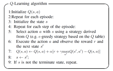Figure 1: -Learning algorithm

The idea of updating the current estimator based on another estimator such as estimate of value of following state as described above is called bootstrap. In the multi-step optimization problem, the bootstrap type learning updates the evaluation value of the current state based on the estimated value of the evaluation value of the next state. Therefore, for example, when the evaluation value is interpreted as the expected value of the reward, even if the problem is complicated, the approximate value can be obtained by repeating the learning.

2.3.  Reflecting the preference of the decision maker

In the multi-objective optimization problem, generally there are multiple Pareto optimal solutions, so it is desirable to rationally select a solution from the Pareto optimal solution set based on the preference structure of the decision maker. On the other hand, it is difficult to model the preference structure of the decision maker mathematically and strictly, so approximate modeling methods have been applied. Representative methods of multi-criteria decision making method include the Analytic Hierarchical Process (AHP)[18], the Analytic Network Process (ANP)[18] and the like. AHP is a method for evaluating relative importance of all standards by decision-makers subjectively making one-pair comparison of pairs of criteria, and so far application to many decision-making problems has been reported. In addition, ANP is a method in which AHP that is a hierarchical structure is expanded to a network structure. However, conventional methods such as AHP and ANP are not mathematically and strictly evaluating the preferences of decision makers, and the obtained solutions are not necessarily the most preferred by decision makers. On the other hand, Multi-Attribute Utility Analysis (MAUT)[18] has been proposed as a method for strictly evaluating and modeling the preference structure of decision makers, but the procedure is complicated and the burden on decision makers is also great.

In this paper, we adopt an interactive method that selects criteria that DM wants to improve against the selected solution, adjusts weight coefficient, and repeats solution improvement until DM accepts as a method to select solutions most preferred by DM among executable Pareto optimal solutions.

The interactive method

It is difficult to identify a function that properly defines and expresses the preference structure of the decision maker. In such a case, by using the interactive method[5] based on limited preference information obtained through dialogue between decision makers and analysts called a preferred solution, it is possible to select the most preferred solution without expressing the preference structure of the decision maker.

In the following multi-objective linear programming problem,

Let be weights of the conflicting objects which the decision maker determines subjectively. The multi-objective linear programming problem is converted into a single objective linear programming problem as follows.

The analyst interactively updates the weights  until the decision maker satisfies with the solution obtained by solving this problem.

3. Hypervolume-Based Multi-Objective Reinforcement Learning

By extending MDP mentioned in Section 2.1 as multi-objective Markov decision process (MOMDP), reinforcement learning can be applied to multi-objective problems. In MOMDP, rewards are given as vectors defined by multi-dimension rather than scalar. That is, given the  objectives  the rewards given are  dimensional vector .Here,  represents transpose.

3.1.  A solution discovery method based on a scalarized objective function

The inner product of the reward vector  given from the environment and the weight coefficient vector  is as follows.­

By using this, it is possible to apply single-objective Q learning to MOMDP. As a method of determining weighting coefficients, AHP, ANP, an interactive method, and the like are conceivable.

3.2.  Multi-objective optimization and Hypervolume

Let  sets of solutions be . Hypervolume [15] represents the volume of the region between a reference point and a region dominated by the solution set in the objective function space. Specifically, it is the surrounded by the boundary formed by solution set and the reference point  necessary to limit the area, therefore Hypervolume can be shown as follows.

Here,  represents the size of the area defined based on reference point  and Pareto solution , and  represents the region formed by the reference point and the Pareto optimal solution set. Here,  represents the union of the areas of Pareto optimal solution set.

Figure 2 shows the solution set of the 4 solutions  in the two-object maximization problem and Hypervolume by reference point . Let  be the area surrounded by thick lines. Hypervolume with four solutions and reference points can be represented by the union of gray area and hatched area.

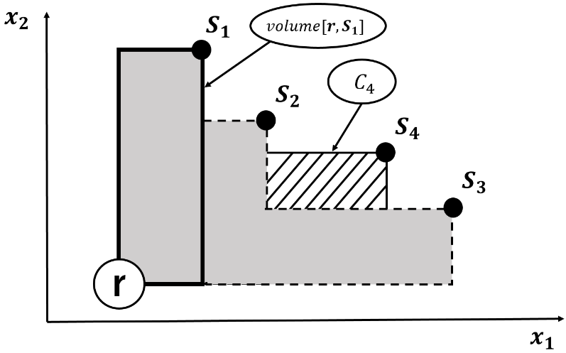Figure 2: Example of Hypervolume

Let consider a new solution  a set of current solution set . Here, let the increased area, that is, the increment of Hypervolume, be the contribution of Pareto solution . Figure 2, the contribution of the Pareto solution  is the area of  which is indicated by the hatched portion. In the objective function space, the Pareto solution in the region where the Pareto solutions are dense is lower the contribution and the contribution becomes higher as the Pareto solution in the region where the Pareto solution are space. Therefore, by selecting solutions with high contribution, it is possible to acquire a wide range of Pareto solution sets without paternity of Pareto solution to some areas.

In this paper, optimization is performed using multi-objective Q-learning which adopts ε-greedy strategy as an action decision policy. In order to obtain a sufficient number of solution candidates, it is necessary to repeat learning according to an decision policy including random action choice such as ε-greedy decision policy. Such that an agent chooses an action with the highest Q-value with probability (1-ε), and the agent randomly choose an action with a low probability ε. However, since the solution that the decision maker most desires is not always the solution with the highest contribution, a decision-making method that selects a solution rationally from the Pareto optimal solution set is necessary other than the method selecting the solution with the highest Hypervolume.

In this paper, we propose a rational decision making method based on the preference structure of decision makers by interactive method from discovered Pareto optimal solution set of the target multi-objective optimization problem. Next section describes the proposed method in detail.

4. Interactive Multi-Objective Reinforcement Learning

In this paper, in order to acquire a sufficient number of Pareto optimal solutions as an optimization method for the multi-objective optimization problem, this paper constructs an efficient solution search method by hypervolume-based multi-objective reinforcement learning. After searching solutions, a solution is selected based on the decision makers’ preference from Pareto optimal solution set by using interactive method. Weight vectors corresponding to the objectives  used in the proposed method are defined as follows.

Here, the algorithm of the proposed method is shown in Figure 3.

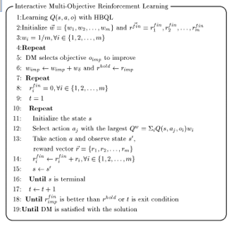Figure 3: The algorithm of the proposed method

By combining such interactive method with hypervolume-based multi-objective reinforcement learning, it became possible to efficiently derive a Pareto optimal solution reflecting the preference of decision makers in multi – step multi – objective optimization problem.

5. Numerical experiments

5.1.  Benchmark Problems and Objectives

This paper conducts numerical experiments using path finding problems as benchmarks of multi-objective optimization problems in continuous value environment in order to confirm the effectiveness of the proposed method. The numerical example is defined on the two-dimensional grid map to which numerical values are assigned to each grid. The numerical value assigned to each grid is a scalar value or a multidimensional vector, and the numerical value at the coordinate  is defined by   for each objective. Also, the total of numerical differences between grids obtained when an agent moves to an adjacent grid is defined as a cost. Specifically, when an agent moves from the grid  to the grid  directry, the numerical difference obtainable for each objective is . The total numerical difference obtained by the agent during single episode is defined as a cost of the corresponding episode. The agent goes on the 2-dimensional grid map and makes a goal, taking into account the following objectives.

• Fewer steps of an episode.
• Smaller cost of an episode.

Detailed settings of the experiments are as follows.

• The agent recognizes the numerical value of the current position and the grid in the eight directions adjacent to the current position.
• The agent obtains a positive reward only when the agent reaches a goal.
• Each step the agent moves, it acquires a negative reward and a non-positive reward based on the numerical difference.
• When the agent tries to go outside the grid map, it acquires a negative reward as a penalty.
• The maximum number of movement of an agent is 10000 steps. If it is not possible to reach the goal during such limitation, learning is interrupted and the next episode is started.
• The maximum number of updates of the weights is 100, and the solution derived by the weights at the time when the number of updates of the weights reaches 100 times, a solution is suggested to the decision maker based on the weights before updating.

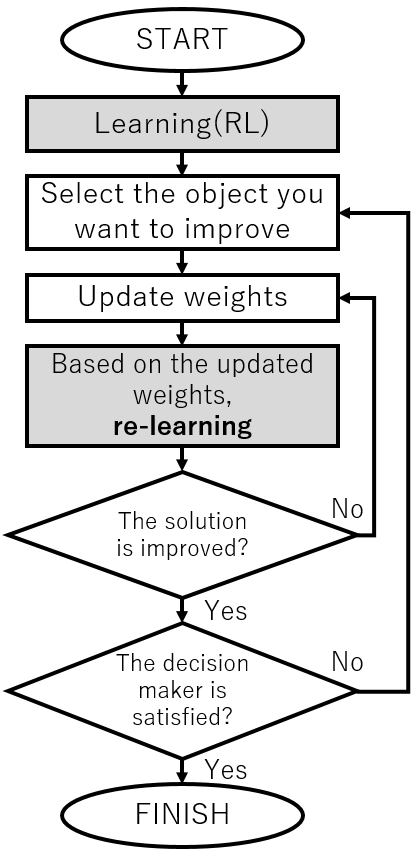Figure 4: Construction of the conventional method

5.2.  The conventional method

In the numerical experiments of this paper, in order to confirm the effectiveness of the proposed method, the experimented result of the proposed method are compared with the result of the conventional method. As a conventional method, single-objective reinforcement learning based on the weighting coefficient method is adopted. This is a method of converting the reward function of the multi-objective optimization problem into a single objective optimization problem by scalarizing the reward function with a weight vector and applying a single-objective Q-learning[19]. Therefore, when the weight vector for scalarizing the reward function is changed, it is necessary to re-learn the Q-value. The flowchart of the proposed method and the comparison method are shown Figure 4 and Figure 5. The differences between these two methods are shown by the gray part.

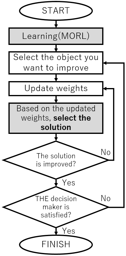Figure 5: Construction of the proposed method

5.3.  Result and Discussion

Three grid maps used for numerical experiments in this paper are shown in Figure 6, ,Figure 8. The lower left green colored cell is the start and the upper right blue colored cell is the goal. Multidimensional numerical values can be allocated on one cell by overlaying these grid maps in  Figure 6, ,Figure 8. Table 1 outlines the numerical experiments of this paper such as combination of grid maps.

Table 1: Outline of Numerical Experiment

Route finding Problem	Minimization objective
#1	(step, )
#2	(step, )
#3	(step )
#4	(step, )

The environment and parameters of this experiment are shown below:

OS:        windows 10 Home 64bit

RAM:    8.00GB

CPU:     intel core-i3 (3.90GHz, 2core, 4thread)

parameters

• wδ=0.1
• rgoal=130
• rwall=-130
• Number of learning episodes = 10000
• At the start of learning, ϵ=0.99 . In addition, after 1000 episodes, ϵ=ϵ×0.97 is calculated every 100 episodes to reduce the value of ϵ .

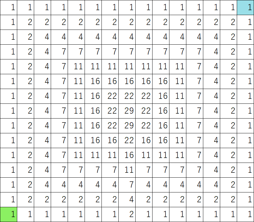Figure 6: Map of fx1

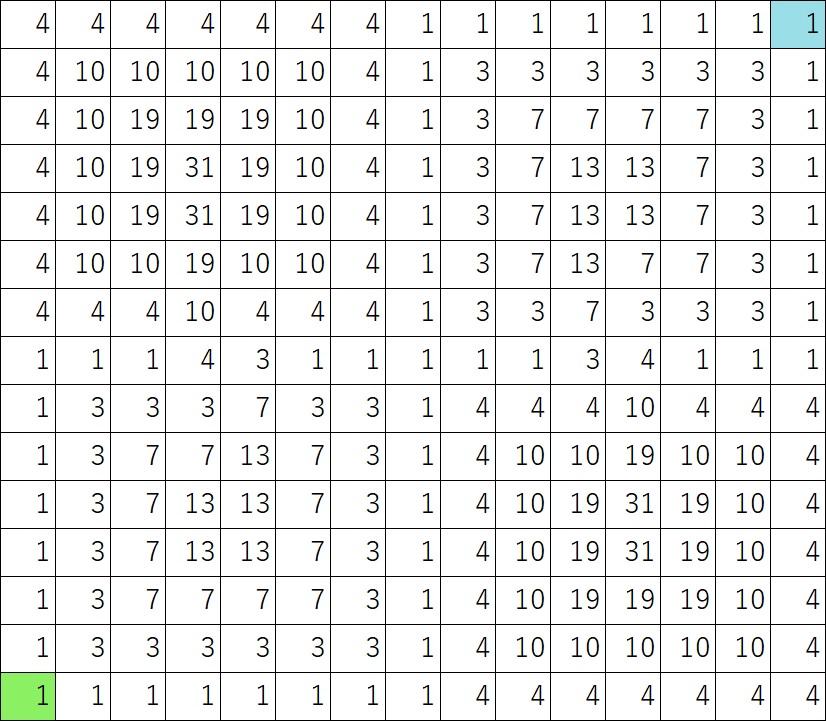Figure 7: Map of fx2

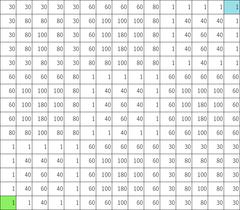Figure 8: Map of fx3

When considering application to realistic multi-step multi-objective optimization problems such as rescue robots and robot cleaners, it was necessary to set weight coefficients of each objective beforehand as in the conventional method so far, it was difficult to select action reflecting the preference of the decision maker. However, by using the method proposed in this paper, it was possible for decision makers to efficiently find the most satisfactory Pareto optimal solutions in the multi – step multi – objective optimization problem.

6. Conclusion

This paper, proposes a multi-objective reinforcement learning with interactive approach to hypervolume-based multi-objective reinforcement learning and confirmed its effectiveness against multi-objective optimization problem in continuous value environments. Conventionally, a method of converting a multi-objective optimization problem into a single-objective problem and applying a single-objective reinforcement learning is common, however, it is difficult to decide the weighting coefficient when converting to a single-objective problem. Also, in order to consider the preference of the decision maker in the weighting coefficient, it is necessary to adjust by single-objective reinforcement learning each time. Such procedure is inefficient in the means of computational cost. Compared to such conventional methods, the proposed method proved to be able to efficiently find Pareto optimal solutions considering the preference of decision makers. As a future task, it is necessary to verify by practical experiment using real machine.

Table  SEQ Table \* ARABIC 2: Improvement by proposed method (Problem #1)

Target	Suggested Solution			Execution time [sec]
	step	costf1	costf2
	18	30	18	3.824
costf1	19	20	22	0.010
Finish			Total	3.834

Table  SEQ Table \* ARABIC 3: Improvement by conventional method (Problem #1)

Target	Suggested Solution			Execution time [sec]
	step	costf1	costf2
	17	30	26	0.888
costf2	18	30	18	3.427
costf1	21	20	22	27.953
step	19	38	38	0.852
costf1	20	30	26	0.849
costf1	25	28	34	4.241
step	17	30	26	0.862
costf1	19	20	22	0.829
Finish			Total	=SUM(ABOVE) 39.901

Table  SEQ Table \* ARABIC 4: Improvement by proposed method (Problem #2)

Target	Suggested Solution			Execution time [sec]
	step	costf2	costf3
	23	54	0	45.220
step	20	54	118	0.013
step	18	48	196	0.010
Finish			Total	=SUM(ABOVE) 45.243

Table  SEQ Table \* ARABIC 5: Improvement by conventional method (Problem #2)

Target	Suggested Solution			Execution time [sec]
	step	costf2	costf3
	23	54	0	1.009
step	21	54	78	15.976
step	20	34	398	6.274
step	19	54	196	24.766
step	18	48	196	0.867
Finish			Total	=SUM(ABOVE) 48.892

Table  SEQ Table \* ARABIC 6: Improvement by proposed method (Problem #3)

Target	Suggested Solution			Execution time [sec]
	step	costf3	costf1
	23	1	30	46.693
Step	20	118	30	0.012
step	17	236	56	0.013
costf1	20	118	30	0.010
Step	17	236	56	0.009
step	14	354	56	0.011
costf1	18	196	42	0.012
costf1	20	118	30	0.010
Step	18	196	42	0.011
step	15	314	42	0.010
costf1	17	236	30	0.010
Finish			Total	=SUM(ABOVE) 46.801

Table  SEQ Table \* ARABIC 7: Improvement by conventional method (Problem #3)

Target	Suggested Solution			Execution time [sec]
	step	costf3	costf1
	23	0	30	0.997
Step	22	238	26	5.546
Step	21	196	42	8.470
Step	20	118	30	20.603
Step	18	196	42	28.715
Step	17	274	42	5.228
costf1	22	276	40	11.209
costf1	22	118	30	4.360
Step	19	196	42	1.692
Step	18	196	42	0.879
step	17	274	42	7.727
costf1	18	354	40	11.889
Step	15	314	42	2.513
costf1	19	356	38	14.884
costf1	17	236	30	7.655
Finish			Total	=SUM(ABOVE) 132.367

Table  SEQ Table \* ARABIC 8: Improvement by proposed method (Problem #4)

Target	Suggested Solution				Execution time [sec]
	step	costf1	costf2	costf3
	23	30	54	0	346.790
step	21	30	54	78	0.015
step	20	30	54	118	0.015
step	20	30	54	118	0.017
step	18	42	48	196	0.014
costf1	20	30	54	118	0.014
step	18	42	48	196	0.013
costf2	17	42	36	354	0.015
costf3	18	42	48	196	0.011
costf3	20	30	54	118	0.013
costf1	20	30	54	118	0.016
step	20	30	54	118	0.016
step	17	30	54	236	0.015
costf3	20	30	54	118	0.012
costf2	18	30	42	276	0.014
costf2	18	30	38	276	0.014
Finish				Total	347.004

Table  SEQ Table \* ARABIC 9: Improvement by conventional method (Problem #4)

Target	Suggested Solution				Execution time [sec]
	step	costf1	costf2	costf3
	23	30	54	0	1.103
step	22	30	50	158	1.937
step	20	42	48	156	4.887
step	19	30	42	276	37.351
step	18	30	54	196	16.966
costf2	21	30	50	276	0.945
step	20	30	54	118	1.835
step	19	42	54	196	1.802
step	18	42	48	196	8.227
costf1	21	36	70	316	1.852
step	20	22	38	238	0.919
step	18	42	48	196	0.919
costf1	26	40	66	316	3.661
costf1	20	30	54	118	0.920
costf2	20	38	38	238	0.934
step	18	42	48	196	1.827
⋮

1.  E. Zitzler and L. Thiele, “Multi-objective optimization using evolutionary algorithms-A comparative case study,” in 5th Int. Conf. Parallel Problem Solving from Nature (PPSN-V), A. E. Eiben, T. B¨ack, M. Schoenauer, and H.-P. Schwefel, Eds. Berlin, Germany: Springer- Verlag, 1998, pp. 292-301.
2.  R. L. Keeney, “Decision analysis: An overview”, Operations research 30 (1982) 803-838. https://doi.org/10.1287/opre.30.5.803
3.  H.-S. Kim and S.-B. Cho, “Application of interactive genetic algorithm to fashion design,” Engineering Applications of Artificial Intelligence, vol. 13, no. 6, pp. 635.644, 2000. http://dx.doi.org/10.1016/S0952-1976(00)00045-2
4.  H. Takagi. “Interactive evolutionary computation: Fusion of the capabilities of EC optimization and human evaluation.” Proceedings of the IEEE, 89(9):1275-1296, September 2001. ISSN 0018-9219. Invited Paper. https://doi.org/10.1109/5.949485
5.  Masatoshi Sakawa , Hitoshi Yano, “An interactive fuzzy satisficing method for multi-objective linear fractional programming problems”, Fuzzy Sets and Systems, v.28 n.2, p.129-144, November 1988. https://doi.org/10.1016/0165-0114(89)90017-1
6.  Tetsuya Higuchi, Yong Liu, and Xin Yao, editors. “Evolvable Hardware”. Springer, New York, 2006.
7.  Sakanashi, H., Iwara, M., Higuchi, T.: “Evolvable hardware for lossless compression of very high resolution bi-level images”. IEEE Proc.-Comput. Digit. Tech., vol. 151, no. 4, (July 2004) 277-286. https://doi.org/10.1049/ip-cdt:20040015
8.  “Lossy/Lossless Coding of Bi-level Images”, ISO/IEC 14492:2001.
9.  H. Tamakoshi, S. Ishii, “Multi-agent reinforcement learning applied to a chase problem in a continuous world”, Artif. Life Robot., vol. 5, no. 4, pp. 202-206, 2001.
10.  R.S. Sutton and A.G. Barto, ”Reinforcement Learning”, MIT Press, 1989.
11.  M. M. Drugan, “Multi-objective optimization perspectives on reinforcement learning algorithms using reward vectors,” proceedings of ESANN, 2015.
12.  S. Natarajan and P. Tadepalli. “Dynamic preferences in Multi-Criteria Reinforcement Learning.” Inproc. of the 22nd International Conference on Machine Learning, 601-608, 2005. https://doi.org/10.1145/1102351.1102427
13.  K. Van Moffaert, M. M. Drugan, and A. Nowe, “Hypervolume-based multi-ojective reinforcement rearning,” 7th International Conference on Evolutionary Multi-Criterion Optimization, 2015.
14.  k. Van Moffaert, A Nowe, “Multi-Objective Reinforcement Learning using Sets of Pareto Dominating Policies.” J. Mach. Learn. Res. 15(1), 3483-3512(2014)
15.  J. Bader and E. Zitzler, “A hypervolume-based optimizer for high-dimensional objective spaces”, Lecture Notes in Economics and Mathematical Systems, Springer, 2009. http://dx.doi.org/10.1007/978-3-642-10354-4_3
16.  K. Deb, S. Agrawal, A. Pratap, and T. Meyarivan, “A fast and elitist multiobjective genetic algorithm: NSGA-II,” IEEE Trans. Evol. Comput., vol. 6, no. 2, pp. 182–197, Apr. 2002.
17.  C. A. Coello Coello and M. S. Lechuga, “MOPSO: A proposal for multiple objective particle swarm optimization,” in Proc. Congr. Evolutionary Computation (CEC’2002), vol. 1, Honolulu, HI, May 2002, pp. 1051–1056.
18.  G.-H. Tzeng and J.-J. Huang, Multiple Attribute Decision Making: Methods and Applications (CRC Press, 2011).
19.  M. Sakawa, I. Nishizaki, H. Katagiri, “Fuzzy Stochastic Multi-objective Programming”, Springer Science Business Media LLC, 2011.

(Click Here)

(Click Here)