1. Introduction

Computing in general shows a growth described by a logistic curve [1] rather than an unlimited exponential curve. Since about 2000, a kind of stalling was experi- enced in practically all components contributing to the single-processor performance, signaling that drastic changes in the approach to computing is needed [2]. However, the preferred way chosen was to continue the traditions of the Single Processor Approach (SPA) [3]: to assemble systems comprising several segregated pro- cessing units, connected in various ways.

The Moore-observation has already been termi- nated in the sense that no more transistors can be added to a single processor, but persists in the sense that more transistors can be placed on a single chip in the form of several cores, complete systems or net- works. In this way the nominal computing performance of processors keeps raising, but the task to produce some payload computing performance remains mostly for the software. However, ”parallel programs … are notoriously difficult to write, test, analyze, debug, and ver- ify, much more so than the sequential versions” [4]. ”The general problem [with parallel programming] is that the basic sentiment seems to go against history. Much of the

*  Ja´nos Ve´gh & Vegh.Janos@gmail.com

progress attributed to the Industrial Revolution is due to using more power for reducing human effort” [5].

The today’s processors comprise a lot of different parallelization solutions [6]. As the result of the devel- opment, ”computers have thus far achieved . . . tremen- dous hardware complexity, a complexity that has grown so large as to challenge the industrys ability to deliver ever- higher performance” [7]. The huge variety of solutions make the efficiency of those systems hard to interpret and measure [8].

In section 2 some issues demonstrate why the present inflexible architectures represent serious is- sues, like bottleneck for parallelized architectures and tremendous non-payload activity during thread-level parallelization.

A (by intention strongly) simplified operating model of parallel operation is presented in section 3. The basis of the section is Amdahl’s law, which is rein- terpreted for the modern computing systems for the purposes of the present study. The technical implementation of parallel systems from sequentially working single-threads using clock signals have their performance limitations as derived in section 4. Both the inherent performance bound (stemming out from the paradigm and the clock-diven electronic technology) and the specific one for supercomputers are discussed. Some aspects of one of the obvious fields of parallel processing: the limitations of supercomputing is discussed in section 5, where short-term prediction for supercomputer performance is also given and the role of different contributions is demonstrated through some issues of brain simulation. Section 6 discusses some possible ways out of the experienced stalling of performance through parallelization.  In section 7 it is concluded that mainly the 70-years old computing paradigm itself (and its consequences: the component and knowledge base) limits the development of com- puting performance through utilizing parallelized se- quential systems.

where we have altogether 4 load operations, 2 multi- plications, and 2 additions. To achieve the maximum parallelism enabled by data dependencies the theoret- ical parallelism assumes the presence of several Pro- cessing Unit (PU)s: (at least) 4 memory access units, 2 multipliers and 2 adders (or equally: an at least 4-issue universal processor). With a such theoretical processor (see Fig. 1, left side) we could load all the four operands in the first machine cycle, to do the multiplications in the second cycle, and to make the addition/subtraction in the last cycle.

In the practical processors, however, the resources are limited and inflexible. In a real (single issue) pro- cessor this task can be solved in 8 cycles, every opera- tion needs a clock cycle.

In a dual-issue processor (see Fig. 1, right side) one issue is able to make calculations, the another one load/store operations. In the real configurations, however, only one memory load operation can be made at a time (mainly due to components manufactured for building SPA computers), so the PUs must wait until all their operands become available. In this case there is only one single clock tick when the two issues work in parallel, and the 8 operations are executed in 7 cycles, in contrast with the theoretical 3 cycles. All this at the expense of (nearly) double hardware (HW) cost.

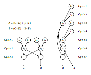Figure 1: Executing the example calculation on a dual issue processor (borrowed from [6])

2. Some architectural issues

The intention with inventing ”computer” was to au- tomate mechanical computing on a single computing resource. Today masses of processors are available for solving a task, and quite typical that the fraction of real computing is much less than the part which imi- tates other functionality through computations (if all you have is a hammer, everything looks like a nail).

2.1. The theoretical parallelism and limits of its technical implementation

When speaking about parallelization, one has to distin- guish the theoretically possible and the technically im- plementable parallelization. Modern processors com- prise several (hidden) processing units, but the efficacy of their utilization is rather poor: the theoretically achievable parallelism in most cases cannot even be approached. To find out the achievable maximum par- allelisation, the different dependencies between the data (as arguments of some operations) shall be consid- ered. Let us suppose we want to calculate expressions (the example is borrowed from [6])

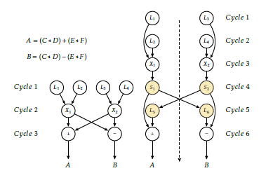Figure 2: Executing the example calculation on a dual core processor (borrowed from [6])

A different idea for distributing the task could be to utilize a dual-core processor, see Fig. 2, right side. Here the multiplications are performed by independent pro- cessors, and also have independent capacity for mak- ing summation and subtraction separately. This (pro- vided that the processors can load their arguments independently) requires only 4 cycles. However, the ”other half” of the result of multiplications belongs to the other processor. The segregated processors can exchange data only through a memory location, so two extra states (in both processors) are inserted for sav- ing and loading the needed data): i.e. the processors execute 12 operations instead of 8 (including 4 slow memory operations), altogether they solve the task in 2*6 clock cycles, instead of 8 (and assume, that the memory will make synchronization, i.e. can assure that reading the intermediate memory locations takes place only when the other party surely wrote that in). That is, (at least) double HW cost, double memory bandwitdh, 50% more instructions and only 25% per- formance increase. Here the additional reason (to the inflexible architecture) is the computing paradigm: the single processor-single process principle.

In both cases the performance increase can be im- plemented at a high price: considerably increased HW cost (and mainly in the latter case: longer, more com- plex software (SW) development). This latter increase gets exponential when solving a real-life program and using more segregated processors. This somewhat the- oretical summary is sufficiently underpinned by expe- riences of practicioners [9].

2.2. Multitasking

With the growing gap between the speed of the pro- cessing and the growing demand for executing com- plex tasks, the need for sharing the single computing resource between processes appeared. The missing features were noticed early [10].

One of the major improvements for enhancing single-processor performance was introducing the reg- ister file. It is practically a different kind of memory, with separate bus, quick access and short address. Al- though the processors could work with essentially less registers [11], today the processors commonly include dozens of registers. However, the processors have been optimized for single-task regime,  so utilizing them for task-level parallelization required serious modifi- cations, both on HW and SW side. What is very advan- tageous for single-thread computing: to have register access time for computations, is very disadvantageous for multitasking: the register contents (or at least part of them) must be saved and restored when switching to another task. The context switching, however, is very expensive in terms of execution time [12]. Also, the too complex and over-optimized architecture con- siderably increases the internal latency time of the processor when used in multi-processor environment: the same architecture cannot be optimized for both work regimes,

Especially in the real-time applications the re- sponse time is very critical. To respond to some ex- ternal signal, the running task must be interrupted, task and processor context saved, task and processor context set for the interrupt, and only after that re- sponding to the external signal can begin. This feature (a consequence of SPA) is especially disadvantageous for cyber-physical systems, networking devices, etc. Synchronizing tasks for those purposes by the operat- ing system (OS) requires tremendous offset work.

The major reason of the problem (among others) is the loose connection between the HW and the SW: in the paradigm only one processor exists, and for a seg- regated processor there is no sense ”to return control”; for the only processor a ”next instruction” must always be available (leading among others to the idea of the ”idle” task is OS, and in a broader sense, to the non energy-proportional operating regime [13]). The HW

interrupts have no information what SW process is ac- tually executed. To mitigate the unwanted effects like priority inversion [14] this instrumental artefact was formalized [15], rather than eliminated by a different HW approach.

3. Amdahl’s Law and model for par- allelized systems

The huge variety of the available parallelization meth- ods, the extremely different technological solutions do not enable to set up an accurate technological model. With the proper interpretation of the Amdahl’s Law, the careful analysis enables to spot essential contri- butions degrading the efficacy of parallelized systems. Despite its simplicity, the model enables to provide a qualitative (or maybe: semi-quantitative) description of the operational characteristics of the parallelized systems, in quite different fields.

3.1. Amdahl’s Law

A half century ago Amdahl [3] called first the atten- tion to that the parallel systems built from segregated sin- gle processors have serious performance limitations. The ”law” he formulated was used successfully on quite different fields [16], sometimes misunderstood, abused and even refuted (for a review see [17]). Despite of that ”Amdahl’s Law is one of the few, fundamental laws of computing” [18], for today it is quite forgotten when analyzing complex computing systems. Although Am- dahl was speaking about complex computing systems, due to its initial analysis about which contributions degrading parallelism can be omitted, today Amdahl’s Law is commonly assumed to be valid for SW only. For today, thanks to the development and huge variety of the technological implementations of parallelized dis- tributed systems, it became obvious that the role of the contributing factors shall be revised.

• Amdahl’s idea

The successors of Amdahl introduced the misconcep- tion that Amdahl’s law is valid for software only and that the non-parallelizable fraction contains something like the ratio of the numbers of the corresponding in- structions or maybe the execution time of the instructions. However, Amdahl’s law is valid for any partly paralleliz- able activity (including computer unrelated ones) and the non-parallelizable fragment shall be given as the ratio of the time spent with non-parallelizable activity to the total time. In his famous paper Amdahl [3] speaks about ”the fraction of the computational load” and explicitly mentions, in the same sentence and same rank, algo- rithmic contributions like ”computations required may be dependent on the states of the variables at each point”; architectural aspects like ”may be strongly dependent on sweeping through the array along different axes on succeeding passes” as well as ”physical problems” like ”propagation rates of different physical effects may be quite different”.

In the present complex parallelized systems his reasoning is still valid: one has to consider the work- load of the complex HW/SW system, rather than of some

the ”sequential-only” fraction. When using several pro- cessors, one of them makes the sequential calculation, the others are waiting (use the same amount of time). So, when calculating the speedup, one calculates

segregated component, and Amdahl’s idea describes par- allelization imperfectness of any kind. Notice that the eligibility of neglecting some component changes with time, technology and conditions. When applied to a particular

case, it shall be individually scrutinized which contribu-

• Deriving the effective parallelization

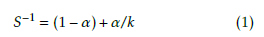
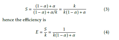
Successors of Amdahl expressed Amdahl’s law with the formula

This explains the behavior of diagram ^S in function of k experienced in practice: the more processors, the lower efficiency. It is not some kind of engineering imperfectness, it is just the consequence of Amdahl’s law. At this point one can notice that ¹ is a linear func- tion of number of processors, and its slope equals to where k is the number of parallelized code fragments,

α is the ratio of the parallelizable part within the total code, S is the measurable speedup. The assumption can be visualized that in α fraction of the running time the processors are executing parallelized code, in (1- α) fraction they are waiting (all but one), or making non-payload activity. That is α describes how much, in average, processors are utilized, or how effective (at the level of the computing system) the parallelization is.

(1   α). Equation (4) also underlines the importance of the single-processor performance: the lower is the number of the processors used in the parallel system having the expected performance, the higher can be the efficacy of the system.

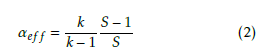
Notice also, that through using (4), the efficiency ^S can be equally good for describing the efficiency of parallelization of a setup, provided that the number of processors is also provided. From (4)For a system under test, where α is not a priory known, one can derive from the measurable speedup

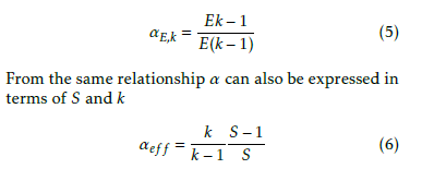which simply means that in the ideal case the actually measurable effective parallelization achieves the the- oretically possible one. In other words, α describes a system the architecture of which is completely known, while α_{ef f} characterizes the performance, which de- scribes both the complex architecture and the actual conditions. It was also demonstrated [19] that α_{ef f} can be successfully utilized to describe parallelized behavior from SW load balancing through measuring

If the parallelization is well-organized (load balanced, small overhead,  right  number  of  processors),  α_{ef f} is very close to unity, so the tendencies can be bet- ter displayed through using (1      α_{ef f} ) (i.e. the non- parallelizable fraction) in the diagrams below.

The importance of this practical term α_{ef f} is un- derlined by that the achievable speedup (performance gain) can easily be derived from (1) as efficacy of the on-chip HW communication to charac- terize performance of clouds.

The value α_{ef f} can also be used to refer back to Am- dahl’s classical assumption even in the realistic case when the parallelized chunks have different lengths and the overhead to organize parallelization is not neg- ligible. The speedup S can be measured and α_{ef f} can be utilized to characterize the measurement setup and conditions, how much from the theoretically possi- ble maximum parallelization is realized. Numerically (1 α_{ef f} ) equals with the f value, established theoreti- cally [20].

The distinguished constituent in Amdahl’s classic analysis is the parallelizable fraction α, all the rest (in- cluding wait time, non-payload activity, etc.) goes into

Correspondingly, the resulting maximum perfor- mance is

• The original assumptions

The classic interpretation implies three¹ essential re- strictions, but those restrictions are rarely mentioned in the textbooks on parallelization:

• the parallelized parts are of equal length in terms of execution time
• the housekeeping (controling parallelization, passing parameters, waiting for termination, ex- changing messages, etc.) has no cost in terms of execution time
• the number of parallelizable chunks coincides with the number of available computing re-

3.2. A simplified model for parallel opera- tion

• The performance losses

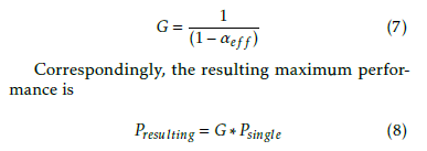
Model of parallel execution sources Essentially, this is why Amdahl’s law represents a theo- retical upper limit for parallelization gain. It is important to notice, however, that a ’universal’ speedup exists only if the parallelization efficiency α is independent from the number of the processors. As will be discussed below, this assumption is only valid if the number of proces- sors is low, so the usual linear extrapolation of the actual performance on the nominal performance will not be valid any more in the case of high number of processors.

• The additional factors considered here

In the spirit of the Single Processor Approach (SPA) the programmer (the person or the compiler) has to or- ganize the job: at some point the initiating proces- sor splits the execution, transmits the necessary pa- rameters to some other processing units, starts their processing, then waits for the termination of started processings; see section 4.1. Real-life programs show sequential-parallel behavior [21], with variable degree of parallelization [22] and even apparently massively parallel algorithms change their behavior during pro- cessing [23]. All these make Amdahl’s original model non-applicable, and call for extension.

As discussed in [24]

• many parallel computations today are limited by several forms of communication and synchro- nization
• the parallel and sequential runtime components are only slightly affected by cache operations
• wires get increasingly slower relative to gates In the followings
• the main focus will be on synchronization and communication; they are kept at their strict ab- solute minimum; and their effect is scrutinized
• the effect of cache will be neglected, and runtime components not discussed separately
• the role of the wires is considered in an extended

Figure 3: The extended Amdahl’s model (strongly sim- plified)

When speaking about computer performance, a mod- ern computer system is assumed, which comprises many sophisticated components (in most cases embed- ding complete computers), and their complex interplay results in the final performance of the system. In the course of efforts to enhance processor performance through using some computing resources in parallel, many ideas have been suggested and implemented, both in SW and HW [6]. All these approaches have different usage scenarios, performance and limitations. Because of the complexity of the task and the lim- ited access to the components, empirical methods and strictly controlled special measurement conditions are used to quantitize performance [8]. Whether a metric is appropriate for describing parallelism, depends on many factors [20, 25, 27].

As mentioned in section 3, Amdahl listed differ- ent reasons why losses in the ”computational load” sense: both the importance of physical distance and using special connection methods will be discussed can occur. To understand the operation of comput- ing systems working in parallel, one needs to extend Amdahl’s original (rather than that of the successors’)

2This separation cannot be strict. Some features can be implemented in either SW or HW, or shared among them, and also some apparently sequential activities may happen partly parallel with each other.

model in such a way, that the non-parallelizable (i.e. apparently sequential) part comprises contributions from HW, OS, SW and Propagation Delay (PD)², and also some access time is needed for reaching the par- allelized system. The technical implementations of different parallelization methods show up infinite vari- ety, so here a (by intention) strongly simplified model is presented. Amdahl’s idea enables to put everything that cannot be parallelized into the sequential-only fraction. The model is general enough to discuss quali- tatively some examples of parallely working systems, neglecting different contributions as possible in the different cases. The model can easily be converted to a technical (quantitative) one and the effect of inter-core communcation can also easily be considered.

• The principle of the measurements

When measuring performance, one faces serious dif- ficulties, see for example [26], chapter 1, both with making measurements and interpreting them. When making a measurement (i.e. running a benchmark) either on a single processor or a system of parallelized processors, an instruction mix is executed many times. The large number of executions averages the rather different execution times [28], with an acceptable stan- dard deviation. In the case when the executed instruc- tion mix is the same, the conditions (like cache and/or memory size, the network bandwidth, Input/Output (I/O) operations, etc) are different and they form the subject of the comparison. In the case when comparing different algorithms (like results of different bench- marks), the instruction mix itself is also different.

Notice that the so called ”algorithmic effects” – like dealing with sparse data structures (which affect cache behavior) or communication between the parallelly running threads, like returning results repeatedly to the main thread in an iteration (which greatly increases the non-parallelizable fraction in the main thread) – manifest through the HW/SW architecture, and they can hardly be separated. Also notice that there are fixed-size contributions, like utilizing time measure- ment facilities or calling system services. Since α_{ef f} is a relative merit, the absolute measurement time shall be long. When utilizing efficiency data from measure- ments which were dedicated to some other goal, a proper caution must be exercised with the interpre- tation and accuracy of the data.

• The formal introduction of the model

The extended Amdahl’s model is shown in Fig. 3. The contributions of the model component XXX to α_{ef f} will be denoted by α^XXX in the followings. Notice the different nature of those contributions. They have only one common feature: they all consume time. The ver- tical scale displays the actual activity for processing units shown on the horizontal scale.

Notice that our model assumes no interaction be- tween the processes running on the parallelized sys- tems in addition to the absolutely necessary minimum: starting and terminating the otherwise independent processes, which take parameters at the beginning and return results at the end.  It can, however, be triv- ially extended to the more general case when processes must share some resource (like a database, which shall provide different records for the different processes), either implicitly or explicitly. Concurrent objects have inherent sequentiality [21], and synchronization and communication among those objects considerably in-

Let us notice that all contributions have a role dur- ing measurement: contributions due to SW, HW, OS and PD cannot be separated, though dedicated mea- surements can reveal their role, at least approximately. The relative weights of the different contributions are very different for the different parallelized systems, and even within those cases depend on many specific factors, so in every single parallelization case a careful analyzis is required.crease [22] the non-parallelizable fraction (i.e. con- tribution (1 − α^SW )), so in the case of extremely large number of processors special attention must be devoted to their role on the efficiency of the application on the parallelized system.

• Access time

Initiating and terminating the parallel processing is usually made from within the same computer, except when one can only access the parallelized computer system from another computer (like in the case of clouds). This latter access time is independent from the parallelized system, and one must properly correct for the access time when derives timing data for the par- allelized system. Failing to do so leads to experimental artefacts like the one shown in Fig. 7. Amdahl’s law is valid only for properly selected computing system. This is a one-time, and usually fixed size time contri- bution.

• Execution time

The execution time Total covers all processings on the parallelized system. All applications, running on a par- allelized system, must make some non-parallelizable activity at least before beginning and after terminat- ing parallelizable activity. This SW activity represents what was assumed by Amdahl as the total sequential fraction³. As shown in Fig. 3, the apparent execution time includes the real payload activity, as well as wait- ing and OS and SW activity. Recall that the execution times may be different [28], [26], [29] in the individual cases, even if the same processor executes the same instruction, but executing an instruction mix many times results in practically identical execution times, at least at model level. Note that the standard deviation of the execution times appears as a contribution to the

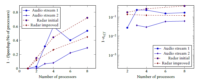Figure 4: Relative speedup (left side) and (1  α_{ef f} ) (right side) values, measured running the audio and radar processing on different number of cores. [31] non-parallelizable fraction, and in this way increases the ”imperfectness” of the architecture. This feature of pro- cessors deserves serious consideration when utilizing a large number of processors. Over-optimizing a pro- cessor for single-thread regime hits back when using it in a parallelized many-processor environment, see also the statistical underpinning in [30].

3.3. fields of application

The developed formalism can be effectively utilized on quite different fields, for more examples see [19].

• Load balancing

The classic field of application is to qualify how effec- tively a parallelized task uses its resources, as shown in Fig. 4. A compiler making load balancing of an orig- inally sequential code for different number of cores is described and validated in paper [31], by running the executable code on platforms having different num- ber of cores. The authors’ first example shows results of implementing parallelized processing of an audio stream manually, with an initial, and a later, more careful implementation. For two different processings of audio streams, using efficiency E as merit enables only to claim a qualitative statement about load bal- ancing, that ”The higher number of parallel processes in Audio-2 gives better results”, because the Audio-2 diagram decreases less steeply, than Audio-1. In the first implementation, where the programmer had no previous experience with parallelization, the efficiency quickly drops with increasing the number of cores. In the second round, with experiences from the first im- plementation, the loss is much less, so 1 E rises less speedily.

Their second example is processing radar signals. Without switching the load balancing optimization on, the slope of the curve 1    E is much bigger. It seems to be unavoidable, that as the number of cores increases, the efficiency (according to Eq. (4)) decreases, even at such low number of cores. Both examples leave the question open whether further improvements are possible or whether the parallelization is uniform in function of the number of cores.

In the right column of the figure (Fig. 10 in [31]) the diagrams show the (1   α_{ef f} ) values, derived from the same data. In contrast with the left side, these values are nearly constant (at least within the mea- surement data readback error) which means that the derived parameter is really characteristic to the system. By recalling (6) one can identify this parameter as the resulting non-parallelizable part of the activity, which even with careful balancing – cannot be distributed among the cores, and cannot be reduced.

In the light of this, one can conclude that both the programmer in the case of audio stream and the com- piler in the case of radar signals correctly identified and reduced the amount of non-parallizable activity: α_{ef f} is practically constant in function of number of cores, nearly all optimization possibilities found and they hit the wall due to the unavoidable contribution of non-parallelizable software contributions. Better parallelization leads to lower (1 α_{ef f} ) values, and less scatter in function of number of cores. The uniformity of the values make also highly probable, that in the case of audio streams further optimization can be done, while processing of radar signals reached its bounds.

• SoC communication method

Another excellent example is shown in Fig. 5. In their work [32] the authors have measured the execution time of some tasks, distributed over a few cores in a System on Chip (SoC). It is worth to notice that the method of calculating (1 α_ef f ) is self-consistent and reliable. In the case of utilizing 2 cores only, the same single communication pair is utilized, independently from the chosen communication method. Correspond- ingly, the diagram lines start at the same (1 α_{ef f} ) value for all communication methods. It is also demon- strated that ”ring” and ”nearest neighbor” methods result in the same communication overhead. Notice also that the (1 − α_{ef f} ) values are different for the two

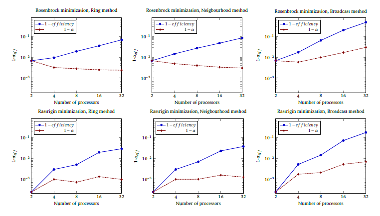Figure 5: Comparing efficiency and α_{ef f} for different communication strategies when running two minimization task on SoC by [32]mathematical methods, which highlights that the same architecture behaves differently when executing a different task.

The commonly used metric (1 ef f iciency) only shows that the efficiency decreases as the number of cores increases. The proposed metric (1 α_{ef f} ) also reveals that while the ”ring” and ”nearest neighbor” methods scale well with the number of cores, in the case of the ”broadcast” method the effective paralleliza- tion gets worse as the number of communicating cores increases. The scatter on the diagrams originate from the short measurement time: the authors focused on a different goal, but their otherwise precise measure- ment can be used for the present goal only with the shown scatter.

• Supercomputer performance design

Utilizing the effective parallelization is important in designing supercomputer architectures, too. Since the resulting performance depends on both the number of processors and the effective parallelization, both quan- tities are correlated with ranking of the supercomputer in Fig. 6. As expected, in TOP50 the higher the rank- ing position is, the higher is the required number of processors in the configuration, and as outlined above, the more processors, the lower (1 α_{ef f} ) is required (provided that the same efficiency is targeted).

In TOP10, the slope of the regression line sharply changes in the left figure, showing the strong com- petition for the better ranking position. Maybe this marks the cut line between the ”racing supercomput-

ers” and ”commodity supercomputers”. On the right figure, TOP10 data points provide the same slope as TOP50 data points, demonstrating that to produce a reasonable efficiency, the increasing number of cores must be accompanied with a proper decrease in value of (1 α_{ef f} ), as expected from (4), furthermore, that to achieve a good ranking a good value of (1   α_{ef f} ) must be provided. Cloud services

In the case of utilizing cloud services (or formerly grids) the parallelized system and the one which in- terfaces user to its application are physically different. These systems differ from the ones discussed above in two essential points: the access and the inter-node connections are provided through using Internet, and the architecture is not necessarily optimized to offer the best possible parallelization. Since the operation of the Internet is stochastic, the measurements cannot be as accurate as in the cases discussed above. The developed formalism, however, can also be used for this case.

The authors of [33] benchmarked some commer- cially available cloud services, fortunately using High Performance Linpack (HPL) benchmark. Their results are shown in Fig. 7. On the left side the efficiency (i.e. RMax ), on the right side (1 − α_{ef f} ) are displayed in func- tion of the processors. They found (as expected) that the efficiency decreases as the number of the proces- sors (nodes) increases. Their one-time measurement

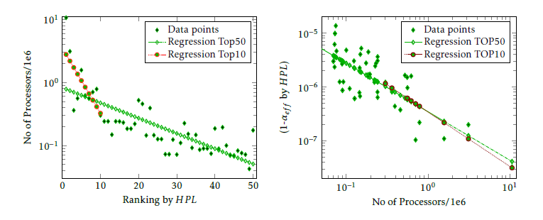Figure 6: Correlation of number of the processors with ranking and effective parallelism with number of processors.

When compared to Fig. 4, one can immediately notice two essential differences. First, that ^RMax is considerably lower than unity, even for very low number of cores. Second, that (1   α_{ef f} ) values steeply decrease as number of cores increases, although the model con- tains only contributions which may only increase as the number of cores increases. Both of those deviations are caused by an instrumental artefact made during bench- marking: when acquiring measurement data also the access time must be compensated for, see Fig. 3.

As discussed above, HPL characterizes the setup comprising processors working in parallel, so the benchmark is chosen correctly. If the time is measured on client’s computer (and this is what is possible using those services), the time Extended is utilized in the cal- culation in place of Total. This artefact is responsible for both mentioned differences. As can be seen from extrapolating the data, the efficiency measured in this way would not achieve 100 % even on a system com- prising only one single processor. Since α_{ef f} measures the average utilization of processors, this foreign con- tribution is divided by the number of processors, so with increasing number of processors this foreign contribution decreases, causing to decrease the calculated value of (1 − α_{ef f} ).

At such low number of processors neither of the contributions depending on the processor number is considerable, so one can expect that in the case of correct measurement (1 α_{ef f} ) would be constant. So, extrapolating graphs (1 α_{ef f} ) to the value correspond- ing to a one-processor system, one can see that for both Edison supercomputer and Azure A series grid (and maybe also Rackspace) the expected value is approach- ing unity (but obviously below it). From the slope of the curve (increasing the denominator 1000 times,

(1 − α_{ef f} ) reduces to 10⁻³) one can even find out that (1 α_{ef f} ) should be around 10⁻³. Based on these data, one can agree with the conclusion that on a good cloud the benchmark High Performance Conjugate Gradients

(HPCG) can run as effectively as on the supercomputer used in the work. However, (1   α_{ef f} ) is about 3 orders of magnitude better for TOP500 class supercomputers, but this makes a difference only for HPL class bench- marks and only at large number of processors.

Note that in the case of AWS clouds and Azure F series the α^OS+SW can be extrapolated to about 10⁻¹, and this is reflected by the fact that their efficiency drops quickly as the number of the cores increases. Interesting to note that ranking based on α_{ef f} is just the opposite of ranking based on efficiency (due to the measurement artefact).

Note also that switching hyperthreading on does not change our limited validity conclusions: both effi- ciency and (1 α_{ef f} ) remains the same, i.e. the hyper- threaded core seems to be a full value core. The place- ment group (PG) option did not affect the measured data considerably.

4. Limitations of parallelization

It is known from the ancient times that there is a mea- sure in things; there are certain boundaries (sunt certi denique fines quos ultra citraque nequit consistere rectum Horace). The different computing-related technical im- plementations also have their limitations [24], conse- quently computing performance itself has its own limi- tations. In parallelized sequential systems an inherent (stemming out from the paradigm and the clock-driven electronic technology) performance limit is derived. The complex parallelized systems are usually qualified (and ranked) through measuring the execution time of some special programs (benchmarks). Since utilizing different benchmarks results in different quantitative features (and ranking [35]), the role of benchmarks is also discussed in terms of the model. It is explained why certain benchmarks result in apparently contro- versial results.

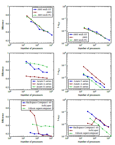Figure 7: Efficiency (left side) and (1   α_{ef f} ) (right side) values for some commercial cloud services. Data from[33] are used

4.1. The inherent limit of parallelization

In the SPA initially and finally  only  one  thread exists, i.e. the minimal absolutely necessary non- parallelizable activity is to fork the other threads and join them again. With the present technology, no such actions can be shorter than one clock period. That is, in this simple case the non-parallelizable fraction will be given as the ratio of the time of the two clock periods to the total execution time. The latter time is a free parameter in describing the efficiency, i.e. the value of

cores are organized into clusters as many supercom- puter builders do, or the processor itself can take over the responsibility of addressing its cores [42]. Depend- ing on the actual construction, the reducing factor can be in the range 10². . . 5 10⁴, i.e the resulting value of (1 α_{ef f} ) is expected to be in the range of 10⁻⁸. . . 2 10⁻⁶.

An operating system must also be used, for prototal benchmarking time (and so does the achievable parallelization gain, too).

The supercomputers, however, are distributed sys- tems. In a stadium-sized supercomputer the distance between processors (cable length) about 100 m can be assumed. The net signal round trip time is cca. 10⁻⁶ seconds, or 10³ clock periods. The presently availableThis dependence is of course well known for super- computer scientists: for measuring efficiency with bet- ter accuracy (and also for producing better α_{ef f} values) hours of execution times are used in practice. For ex- ample in the case of benchmarking the supercomputer Taihulight [36] 13,298 seconds benchmark runtime was used; on the 1.45 GHz processors it means 2 10¹³ clock periods. This means that (at such benchmarking time) the inherent limit of (1 α_{ef f} ) is 10⁻¹³ (or equiv- alently the achievable performance gain is 10¹³). In the followings for simplicity 1.00 GHz processors (i.e. 1 ns clock cycle time) will be assumed.

network interfaces have 100. . . 200 ns latency times, and sending a message between processors takes time in the same order of magnitude. This also means that making better interconnection is not a bottleneck in en- hancing performance of large-scale supercomputers. This statement is underpinned also by statistical considera- tions [30].

Taking the (maybe optimistic) value 2∗10³ clock petection and convenience. If one considers the context switching with its consumed 2 10⁴ cycles [12], the absolute limit is cca. 5 10⁻⁸, on a zero-sized super- computer. This is why Taihulight runs the actual com- putations in kernel mode [42].

It is crucial to understand that the decreasing effi– ciency (see (4)) is coming from the computing paradigm itself rather than from some kind of engineering imperfect- ness. This inherent limitation cannot be mitigated without changing the computing paradigm.

Although not explicitly dealt with here, notice that the data exchange between the first thread and the other ones also contribute to the non-parallelizable fraction and tipically uses system calls,  for details see [22, 44] and section 4.2. supercomputer. This also means that the expectations against the absolute performance of supercomputers are excessive: assuming a 10 Gflop/s processor, the achievable absolute nominal performance is 10¹⁰*10¹⁰, i.e. 100 EFlops. In the feasibility studies an analysis for whether this inherent performance bound exists

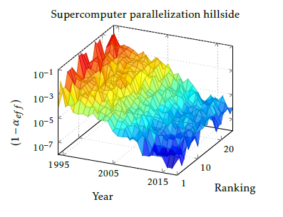Figure 8: The Top500 supercomputer parallelization efficiency in function of the year of construction and the actual ranking. The (1 − α) parameter for the past Another major issue arises from the computing paradigm SPA: only one computer at a time can be ad- dressed by the first one. As a consequence, minimum as many clock cycles are to be used for organizing the parallel work as many addressing steps required. Ba- sically, this number equals to the number of cores in the supercomputer, i.e. the addressing in the TOP10 positions typically needs clock cycles in the order of 5 ∗ 10⁵. . . 10⁷; degrading the value of (1 − α_{ef f} ) into the range 10⁻⁶. . . 2 10⁻⁵. Two tricks may be used to reduce the number of the addressing steps: either the derived using the HPL benchmark.

4.2. Benchmarking the performance of a complex computing system

As discussed above, measuring the performance of a complex computing system  is  not  trivial  at  all. Not  only  finding  the  proper  merit  is  hard,  but also the ”measuring device” can basically influence the measurement. The importance of selecting the proper merit and benchmark can be easily understood

through utilizing the model and the well-documented benchmark measurements of the supercomputers.

As experienced in running the benchmarks HPL and HPCG [45] and explained  in  connection  with Fig. 13, the different benchmarks produce different payload performance values and computational effi- ciencies on the same supercomputer. The model pre- sented in Fig. 3 enables to explain the difference.

The benchmarks, utilized to derive numerical pa- rameters for supercomputers, are specialized programs, which run in the HW/OS environment provided by the supercomputer under test. Two typical fields of their utilization: to describe the environment supercom- puter application runs in, and to guess how quickly an application will run on a given supercomputer.

Performance gain of supercomputers, Top 500 1st-3rd distort HW+OS contribution as little as possible, i.e. the SW contribution must be much lower than the HW+OS contribution. In the case of supercomputers, the benchmark HPL is used for this goal since the be- ginning of the supercomputer age. The mathematical behavior of HPL enables to minimize SW contribution,

i.e. HPL delivers the possible best estimation for α^HW+OS .

If the goal is to estimate the expectable behavior of an application, the benchmark program should imi- tate the structure and behavior of the application. In the case of supercomputers, a couple of years ago the benchmark HPCG has been introduced for this goal, since ”HPCG is designed to exercise computational and data access patterns that more closely match a different and broad set of important applications, and to give incen- tive to computer system designers to invest in capabilities that will have impact on the collective performance of these applications” [45]. However, its utilization can be mis- leading: the ranking is only valid for the HPCG applica- tion, and only utilizing that number of processors. HPCG seems really to give better hints for designing super- computer applications⁵, than HPL does. According to our model, in the case of using the HPCG benchmark, the SW contribution dominates⁶, i.e. HPCG delivers

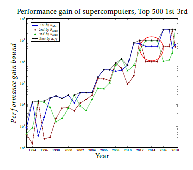Figure 9: The trend of the development of computing performance gain in the past 25 years, based on the first three (by R_Max) and the first (by (1 α)) in the year of construction. Data derived using the HPL bench- mark. A saturation effect around 10⁷ is expressed.

The (apparently) sequential fraction (1   α_{ef f} ), as it is obvious from our model, cannot distinguish be- tween the (at least apparently) sequential processing time contributions of different origin, even the SW (in- cluding OS) and HW sequential contributions cannot be separated. Similarly, it cannot be taken for sure that those contributions sum up linearly. Different benchmarks provide different SW contributions to the non-parallelizable fraction of the execution time (re- sulting in different efficiencies and ranking [35]), so comparing results (and especially establishing rank- ing!) derived using different benchmarks shall be done with maximum care. Since the efficiency depends heavily on the number of cores, different configurations shall be compared using the same benchmark and the same number of processors (or same R_Peak).

If the goal is to characterize the supercomputer’s HW+OS system itself, a benchmark program should puter applications.

Supercomputer community has extensively tested the efficiency of TOP500 supercomputers when bench- marked with HPL and HPCG [45]. It was found that the efficiency (and R_Max) is typically 2 orders of magni- tude lower when benchmarked with HPCG rather than with HPL, even at relatively low number of processors.

5. Supercomputing

In supercomputing the resulting payload computing performance is crucial and the number of the pro- cessors, their single-processor performance and the speed of their interconnection are critical resources. As today a ”gold rush” is experienced with the goal to achieve the dream limit of 1 Eflop/s (10¹⁸ f lop/s) [46], the section scrutinizes the feasibility of achieving that goal. Through applying the model to different kinds of large-scale sequential-parallel computing systems it is shown that such systems require to understand the role and dominance of the contributions of quite different kinds to the performance loss and that the improperly designed HW/SW cooperation provides direct evidence about the existence of the performance bound. The well-documented, strictly controlled mea- surement database [48] enables to draw both retrospec- tive statistical conclusions on the logic of development behind the performance data, as well as to make pre- dictions for the near future about the performance of supercomputers and its limitations.

5This is why for example [47] considers HPCG as ”practical performance”.

6 Returning calculated gradients requires much more sequential communication (unintended blocking).

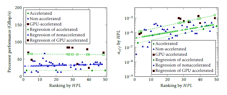Figure 10: Correlation of performance of processors using accelerator and effective parallelism with ranking, in 2017. The left figure shows that utilizing GPU accelerators increases single-processor performance by a factor of 2. . . 3, but as the right side demonstrates, at the price of increasing the non-parallelizable fraction.

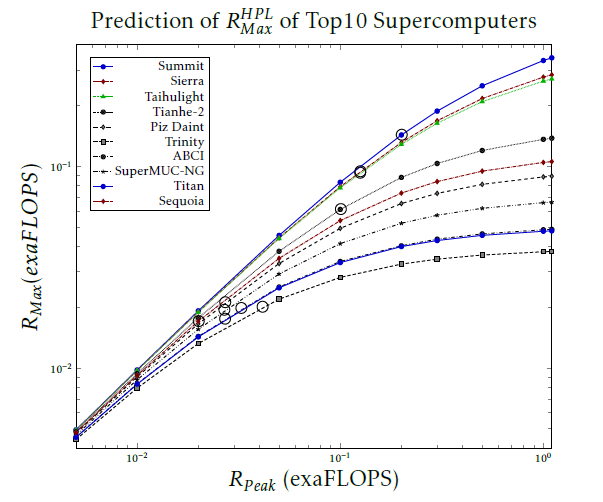Figure 11: Dependence of payload supercomputer performance on the nominal performance for the TOP10 supercomputers (as of November 2018) in case of utilizing the HPL benchmark. The actual positions are marked by a bubble on the diagram lines.

5.1. Describing the development of super- computing

One can assume that all configurations are built with the actually available best technology and components, and only the really best configurations can be found in circles of TOP lists. The large number of configurations in the rigorously controlled database TOP500 [48] enables to draw reliable conclusions, although with considerable scattering. Fig. 8 depicts the calculated

Fig. 11 shows the virtual payload performance in the function of the nominal performance for the TOP10 su- percomputers (as of November 2018). Notice that the predictions are optimistic, because the performance breakdown shown in Fig. 13 is not included. Even with that optimistic assumption, the 1 Eflop/s pay- load performance cannot be achieved with the present technology and paradigm.

Development of R^HPL for the PizDaint Supercomputer (1 α_{ef f} ) for the past 26 years and the first 25 comput- ers in the TOP500 list.

Fig. 8 explicitly shows signs of reaching a ”flat sur- face” in values of (1 α_{ef f} ) in the past few years. This effect can be more clearly studied if considering the TOP3 supercomputers only. Fig. 9 depicts the per- formance gain (see (7)) of supercomputers for their 26-years history. As seen, symptoms of stalling of the parallelized performance appeared in 2012: in three adjacent years the payload performance gain of the TOP3 supercomputers remained at the same value. With the appearance of Taihulight in 2016 apparently a by an order of magnitude higher performance gain has shined up.   However,  it is just the consequence of using the ”cooperative computing” [42], the rest of world remains under that limiting stalling value. The new world champion in 2018 could conquer the slot #1 only due to its higher (accelerator-based) single-processor performance, rather than the enhanced effec- tive parallelization (although its clustering played an important role in keeping it in good condition).

5.2. Predictions of supercomputer perfor- mance for the near future

As Eq. (8) shows, the resulting performance can be in- creased by increasing either the single processor perfor- mance or the performance gain. As the computational density cannot be increased any more [49, 50], some kind of accelerator is used to (apparently) increase the single processor performance. The acceleration, however, can also contribute to the non-parallelizable fraction of the computing task.

Fig. 10 shows how utilizing Graphic Processing Unit (GPU) acceleration is reflected in parameters of the TOP50 supercomputers. As the left side of the figure displays, the GPU really increases the single- processor performance by a factor of 2. . . 3 (in accor- dance with [51]), but at the same time increases the value of (1 α_{ef f} ). The first one is a linear multiplier, the second one is an exponential divisor. Consequently, at low number of cores it is advantageous to use that kind of acceleration, while at high number of cores it is definitely disadvantageous.

Having the semi-technical model ready, one can es- timate how the computing performance will develop in the coming few years. Assuming that the designers can keep the architecture at the achieved performance gain, changing virtually the number of processors one can estimate how the payload performance changes when adding more cores to the existing TOP10 constructions.

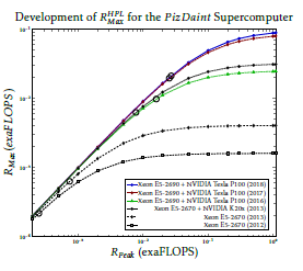Figure 12: Dependence of the predicted payload perfor- mance of supercomputer Piz Daint in different phases of the development, with the prediction based on the actual measured efficiency values. The actual positions are marked by bubbles on the diagram lines.

The accuracy of the short-term prediction can be estimated from Fig. 12. Fortunately, supercomputer Piz Daint has a relatively  long  documented  history in the TOP500 database [48]. The publishing of the results of the development has started in year 2012. In the next year the number of the processors has changed by a factor of three, and the parallelization efficiency considerably improved by the same factor, although presumably some hardware efficacy improve- ments have also occurred. Despite this, the predicted performance improvement is quite accurate. (unfor- tunately, two parameters have been changed between two states reported to the list, so their effect cannot be qualified separately.) In year 2013 GPU acceleration with K20 have been introduced, and the number of processors have been increased by a factor of four. The resulting effect is a factor of 10 increase in both the payload performance and the nominal performance. Probable a factor of 2.5 can be attributed to the GPU, which value is in good agreement with the values re- ceived in[51, 30], and a factor of 4 to the increased number of cores. The designers were not satisfied with the result, so they changed to TESLA P100. Notice that the change to a more advanced type of GPU results in a slight fallback relative to the prediction in the expected value of R_Max : copying between a bigger GPU memory and the main memory increases the non parallizable

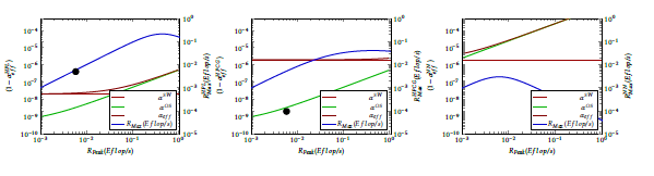Figure 13: Contributions (1 − α^X    ) to (1 − α^total ) and max payload performance R_Max of a fictive supercomputer(P = 1Gf lop/s @ 1GHz) in function of the nominal performance. The blue diagram line refers to the right hand scale (R_Max values), all others ((1 − α^X  ) contributions) to the left scale.  The leftmost figure illustrates the behavior measured with benchmark HPL. The looping contribution becomes remarkable around 0.1 Eflops, and breaks down payload performance when approaching 1 Eflops. The black dot marks the HPL performance of the computer used in works [53, 55]. In the middle figure the behavior measured with benchmark HPCG is displayed. In this case the contribution of the application (thin brown line) is much higher, the looping contribution (thin green line) is the same as above. As a consequence, the achievable payload performance is lower and also the breakdown of the performance is softer. The black dot marks the HPCG performance of the same computer. The rightmost figure demonstrates what happens if the clock cycle is 5000 times longer: it causes a drastic decrease in the achievable performance and strongly shifts the performance breakdown toward lower nominal performance values. The figure is purely illustrating the concepts; the displayed numbers are somewhat similar to the real ones.

contribution, which cannot be counterbalanced even by the two times more cores. Finally, the constructors upgraded also the processor (again changing two pa- rameters at a time), but the twice more processors and the new accelerator produced only twice more perfor- mance. The upgrade in 2018 accurately predicted by the diagram. As the diagram lines in Fig. 12 accurately display the resulting values of the later implementa- tion if no changes in the architecture (the efficiency) happens, one can rely to the estimations for predicting future values displayed in Fig. 11, provided that no ar- chitectural changes (or changes in the paradigm) occur during the development.

5.3. What factors dominate the perfor- mance gain

As discussed above, different goals can be targeted with the parallelized sequential HW/SW systems. Ac- cordingly, different factors dominate in limiting the computational performance. The case of simulating large neural networks is a very good example how the dominance of the different factors changes with the actual conditions.

The idea of simulating neural activity in a way that processors are used to provide the computing facility for solving partial differential equations, seems to be a good idea, as well as to utilize paralelly running SW threads to imitate neural activity of large networks. However, utilizing parallelized sequential systems for that goal implies all limitations discussed above.

As discussed in details in [52], two of the men- tioned effects can become dominating in those applica- tions. Since the operating time scale of the biological

networks lies in the msec range, brain simulation appli- cations commonly use integration time about 1 ms [53]. Since the threads running in parallel need to be syn- chronized (i.e. they must be put back on the same biological time scale, in order to avoid working with ”signals from the future”), quietly and implicitly a 1 ms ”clock signal” is introduced. Since this clock period is million times longer than the typical clock period in digital computers, its dominance is seriously pro- moted in producing non-payload overhead. This im- plicit clock signal has the same limiting effect for both the many-thread simulation and the special-purpose HW brain simulator [54]. This is why the special HW brain simulator cannot outperform the many-thread version SW running on a general-purpose supercom- puter.

The other field-specific effect is that the process- ing speed is too quick and the storage capacity is too large for simulating biological systems in an economic way, so the same core is utilized to simulate several neurons (represented by several threads). This method of solution however needs several context switchings within the same core, and since the context switchings are rather expensive in terms of execution time [12], the overhead part of the process amounts to 10% [53], and the 0.1 value of (1 α_{ef f} ) competes for dominance with the improperly selected clock period. This is the reason why the many-thread based simulation cannot scale above a few dozens of thousands of neurons [55]. (At the same time, the analog simulators achieve thou- sands time better performance and scaling.)

It is worth to have look at Fig. 13. The thick blue line shows the dependence of the payload performance on the nominal performance under different conditions and refers to the right side scale. The leftmost figure shows the case of running the benchmark HPL in some fictive (but somewhat similar to Taihulight) supercomputer. The middle figure shows how a typical computation (modelled by the benchmark HPCG, uti- lizing intensively communication among the threads) leads to strong degradation of payload performance at higher nominal performances. HPCG is in its behav- ior greatly similar to AI applications. These real-life applications show also smeared maximum behavior (compared to those of the benchmark HPL).

On the rightmost figure the clock signal is 5,000 times higher, modeling the ”hidden clock signal”. In this case the performance degradation is much more expressed, and also the breakdown of the performance has been measured [55].

6. How to proceed after reaching limits of parallelization

Today the majority of leading researchers agree that computing (and especially: the computing paradigm) needs renewal (for a review see [56]), although there is no commonly accepted idea for a new paradigm. After the failure of supercomputer Aurora (A18) project it became obvious that a processor optimized for SPA regime cannot be optimal at the same time for paral- lelized sequential regime.

Intel learned the lesson and realized that exa-scale computing needs a different architecture. Although Intel is very cautious with discovering its future plans, especially the exa-scale related ones[57], they already dropped the X86 line[58]. Their new patent [59] at- tempts to replace the conventional instruction-driven architecture by a data-driven one. However, a serious challenge will be to eliminate the overhead needed to frequently reconfigure the internals of the processor for the new task fraction and it is also questionable that emulating the former X86 architecture (obviously from code compatibility reasons) enables to reduce the inherent overhead coming from that over-complex single-processor oriented architecture. The new and ambitious player in Europe [39, 60], however, thinks that some powerful architecture (although even the processor type is not selected) can overcome the theo- retical and technological limits without changing the paradigm. That is, there are not much ”drastically new” ideas on board.

As discussed above, from the point of view of paral- lelism the inherently sequential parts of any HW/SW system form a kind of overhead. The happenings around parallelised sequential processing systems val- idate the prophecy of Amdahl: The nature of this over- head [in parallelism] appears to be sequential so that it is unlikely to be amenable to parallel processing tech- niques. Overhead alone would then place an upper limit on throughput . . . , even if the housekeeping were done in a separate processor [3]

As Amdahl in 1967(!) warned: the organization of a single computer has reached its limits and that truly sig-

nificant advances can be made only by interconnection of a multiplicity of computers in such a manner as to permit co- operative solution [3]. Despite that warning, even today, many-processor systems, including supercomputers, distributed systems and many-core processors as well, comprise many single-processor systems, (rather than ”cooperating processors” as envisioned by Amdahl). The suggested solutions typically consider segregated cores, based on SPA components and use programmed communication, like [61].

There are some exceptions, however: solutions like [62, 63] transfer control between (at Instruction Set Architecture (ISA) level) equivalent cores, but un- der SW control. Direct connection between cores exists only in [42], also under SW control. This processor has kept the supercomputer Taihulight in the first slot of the TOP500 list [48] for two years. Optimizing this direct (non-memory related) data transfer resulted in drastic changes [43] in the executing of the HPCG benchmark (mitigating the need to access memory de- creases the sequential-only part). Unfortunately, the architectures with programmed core-to-core connec- tion are not flexible enough: the inter-core register-to- register data transfer must be programmed in advance by the programmer. The need for solving architectural inflexibility appeared, in the form of ”switchable topol- ogy” [64]. The idea of ”outsourcing” (sending compute message to neighboring core) [65] also shined up. Both suggestions without theoretical and programming sup- port.

A different approach can be to use a radically new (or at least a considerable generalization of the old) com- puting paradigm. That radically new paradigm at the same time must provide a smooth transition from the present age to the new one, as well as co-existence for the transition period. The idea of utilizing Explicitly Many-Processor Approach (EMPA) [66] seems to fulfill those requirements, although it is in a very early stage of development.

The technology of manufacturing processors (mainly the electronic component density) as well as the requirements against its utilization have consider- ably changed since the invention of the first computer. Some of the processing units (the cores within a pro- cessor) are in close proximity, but this alone, without cooperation is not sufficient. Even utilizing synergis- tic cell processors [67] did not result in breakthrough success. Utilizing cooperation of processors in close proximity [42], however, resulted in the best effective parallelism up to now. Establishing further ways of cooperation (like distributing execution of task frag- ments to cooperating cores in close proximity [66, 68]), however, can considerably enhance the apparent per- formance through decreasing the losses of paralleliza- tion.

7. Summary

The parallelization of otherwise sequential processing has its natural and inherent limitations, does not meet the requirements of modern computing and does not provide the required flexibility. Although with de- creasing efficiency, for part of applications sufficiently performable systems can be assembled and with some tolerance and utilizing special SW constraints, the real- time needs can be satisfied. In the case of extremely large processing capacity, however, bounds of the par- allelized sequential systems are faced. For developing the computing performance further, the 50-years old idea about making systems comprising cooperating processors must be renewed. The need for cooperative computing is evident and its feasibility was convincingly demon- strated by the success of the world’s first really coopera- tive processor [42]. An extension [66] to the computing paradigm, that considers both the technological state- of-the-art and the expectations against computing, was also presented and some examples of its advantageous features were demonstrated.

Conflict of Interest

The authors declare no conflict of interest.

Acknowledgment

Project no. 125547 has been im- plemented with the support provided from the Na- tional Research, Development and Innovation Fund of Hungary, financed under the K funding scheme.

1.  P. J. Denning, T. Lewis, Exponential Laws of Computing Growth, COMMUN ACM (2017) 54–65doi:DOI:10.1145/ 2976758.
2.  S. H. Fuller and L. I. Millett, Computing Performance: Game Over or Next Level?, Computer 44/1 (2011) 31-.38.
3.  G. M. Amdahl, Validity of the Single Processor Approach to Achieving Large-Scale Computing Capabilities, in: AFIPS Conference Proceedings, Vol. 30, 1967, pp. 483–485. doi: 10.1145/1465482.1465560.
4.  J. Yang et al., Making Parallel Programs Reliable with Stable Multithreading COMMUN ACM 57/3(2014)58-69
5.  U. Vishkin, Is Multicore Hardware for General-Purpose Parallel Processing Broken?, COMMUN ACM, 57/4(2014)p35
6.  K. Hwang, N. Jotwani, Advanced Computer Architecture: Parallelism, Scalability, Programmability, 3rd Edition, Mc Graw Hill, 2016.
7.  Schlansker, M.S. and Rau, B.R. EPIC: Explicitly Parallel Instruction Computing, Computer 33(2000)37–45
8.  D. J. Lilja, Measuring Computer Performance: A practitioner’s guide, Cambridge University Press, 2004.
9.  Singh, J. P. et al, Scaling Parallel Programs forMultiprocessors: Methodology and Examples, Computer 27/7(1993),42–50
10.  Arvind and Iannucci, Robert A., Two Fundamental Issues in Multiprocessing 4th International DFVLR Seminar on Foundations of Engineering Sciences on Parallel Computing in Science and Engineering (1988)61–88
11.  Mahlke, S.A. and Chen, W.Y. and Chang, P.P. and Hwu, W.- M.W., Scalar program performance on multiple-instructionissue processors with a limited number of registers Proceedings of the Twenty-Fifth Hawaii International Conference on System Sciences (1992)34 – 44
12.  D. Tsafrir, The context-switch overhead inflicted by hardware interrupts (and the enigma of do-nothing loops), in: Proceedings of the 2007 Workshop on Experimental Computer Science, ExpCS ’07, ACM, New York, NY, USA, 2007, pp. 3–3. URL http://doi.acm.org/10.1145/1281700.1281704
13.  Luiz Andr Barroso and Urs Hlzle, The Case for Energy- Proportional Computing Computer 40(2007)33–37
14.  ”Babaolu, zalp and Marzullo, Keith and Schneider, Fred B.”, ”A formalization of priority inversion” Real-Time Systems, 5/4(1993)285303
15.  ”L. Sha and R. Rajkumar and J.P. Lehoczky”, ”Priority inheritance protocols: an approach to real-time synchronization” IEEE Transactions on Computers, 39/4(1990)1175–1185
16.  S. Krishnaprasad, Uses and Abuses of Amdahl’s Law, J. Comput. Sci. Coll. 17 (2) (2001) 288–293. URL http://dl.acm.org/citation.cfm?id=775339. 775386
17.  F. D´evai, The Refutation of Amdahl’s Law and Its Variants, in: O. Gervasi, B. Murgante, S. Misra, G. Borruso, C. M. Torre, A. M. A. Rocha, D. Taniar, B. O. Apduhan, E. Stankova, A. Cuzzocrea (Eds.), Computational Science and Its Applications – ICCSA 2017, Springer International Publishing, Cham, 2017, pp. 480–493.
18.  J. M. Paul, B. H. Meyer, Amdahl’s Law Revisited for Single Chip Systems, INT J of Parallel Programming 35 (2) (2007) 101–123.
19.  J. V´egh, P. Moln´ar, How to measure perfectness of parallelization in hardware/software systems, in: 18th Internat. Carpathian Control Conf. ICCC, 2017, pp. 394–399.
20.  A. H. Karp, H. P. Flatt, Measuring Parallel Processor Performance, COMMUN ACM 33 (5) (1990)Inherent Sequentiality: 2012 539–543. doi:10.1145/78607.78614.
21.  F. Ellen, D. Hendler, N. Shavit, On the Inherent Sequentiality of Concurrent Objects, SIAM J. Comput. 43 (3) (2012) 519536.
22.  L. Yavits, A. Morad, R. Ginosar, The effect of communication and synchronization on Amdahl’s law in multicore systems, Parallel Computing 40 (1) (2014) 1–16.
23.  K. Pingali, D. Nguyen, M. Kulkarni, M. Burtscher, M. A. Hassaan, R. Kaleem, T.-H. Lee, A. Lenharth, R. Manevich, M. M´endez-Lojo, D. Prountzos, X. SuiThe Tao of Parallelism in Algorithms, SIGPLAN Not. 46 (6) (2011) 12–25.
24.  I. Markov, Limits on fundamental limits to computation, Nature 512(7513) (2014) 147–154.
25.  Sun, Xian-He and Gustafson, John L., Toward a Better Parallel Performance Metric Parallel Comput., 17/10-11(1991)1093– 1109
26.  D.A. Patterson and J.L. Hennessy, Computer Organization and design. RISC-V Edition, (2017) Morgan Kaufmann
27.  S. Orii, Metrics for evaluation of parallel efficiency toward highly parallel processing ”Parallel Computing ” 36/1(2010)16–25
28.  P. Moln´ar and J. V´egh, Measuring Performance of Processor Instructions and Operating System Services in Soft Processor Based Systems. 18th Internat. Carpathian Control Conf. ICCC (2017)381–387
29.  Randal E. Bryant and David R. O’Hallaron, Computer Systems: A Programmer’s Perspective (2014) Pearson
30.  J. V´egh, Statistical considerations on limitations of supercomputers, CoRR abs/1710.08951.
31.  W. Sheng et al., A compiler infrastructure for embedded heterogeneous MPSoCs Parallel Computing volume = 40/2(2014)51-68
32.  L. de Macedo Mourelle, N. Nedjah, and F. G. Pessanha, Reconfigurable and Adaptive Computing: Theory and Applications. CRC press, 2016, ch. 5: Interprocess Communication via Crossbar for Shared Memory Systems-on-chip.
33.  Mohammadi, M. and Bazhirov, T., Comparative Benchmarking of Cloud Computing Vendors with High Performance Linpack Proceedings of the 2nd International Conference on High Performance Compilation, Computing and Communications (2018)1–5
34.  E. Wustenhoff and T. S. E. Ng, Cloud Computing Benchmark(2017) https://www. burstorm.com/price-performance-benchmark/ 1st-Continuous-Cloud-Price-Performance-\ Benchmarking.pdf
35.  IEEE Spectrum, Two Different Top500 Supercomputing Benchmarks Show Two Different Top Supercomputers, https://spectrum.ieee.org/tech-talk/computing/ hardware/two-different-top500-supercomputing-\ benchmarks-show-two-different-top-\supercomputers (2017).
36.  J. Dongarra, Report on the Sunway TaihuLight System, Tech. Rep. Tech Report UT-EECS-16-742, University of Tennessee Department of Electrical Engineering and Computer Science (June 2016).
37.  Robert F. Service, Design for U.S. exascale computer takes shape, Science, 359/6376(2018)617–618
38.  US DOE, The Opportunities and Challenges of Exascale Computing, https://science.energy.gov/˜/media/ascr/ ascac/pdf/reports/Exascale_subcommittee_report.pdf (2010).
39.  European Commission, Implementation of the Action Plan for the European High-Performance Computing strategy, http://ec.europa.eu/newsroom/dae/document.cfm? doc_id=15269 (2016).
40.  Extremtech Japan Tests Silicon for Exascale Computing in 2021. https://www.extremetech.com/computing/ 272558-japan-tests-silicon-for-exascale-\ computing-in-2021
41.  X Liao, Kaiet al Moving from exascale to zettascale computing: challenges and techniques. Frontiers of Information Technology & Electronic Engineering 567 19(10) pp: 1236–1244 (2018)
42.  F. Zheng, H.-L. Li, H. Lv, F. Guo, X.-H. Xu, X.-H. Xie, Cooperative computing techniques for a deeply fused and heterogeneous many-core processor architecture, Journal of Computer Science and Technology 30 (1) (2015) 145–162.
43.  Ao, Yulong et al Performance Optimization of the HPCG Benchmark on the Sunway TaihuLight Supercomputer ACM Trans. Archit. Code Optim. 15/1(2018)1-20
44.  S. Eyerman, L. Eeckhout, Modeling Critical Sections in Amdahl’s Law and Its Implications for Multicore Design, SIGARCH Comput. Archit. News 38 (3) (2010) 362–370.
45.  HPCG Benchmark, http://www.hpcg-benchmark.org/ (2016).
46.  J. Dongarra, The Global Race for Exascale High Performance Computing(2017) http://ec.europa.eu/newsroom/ document.cfm?doc_id=45647
47.  Tim Dettmers, The Brain vs Deep Learning Part I: Computational Complexity Or Why the Singularity Is Nowhere Near (2015) http://timdettmers.com/2015/07/ 27/brain-vs-deep-learning-singularity/
48.  TOP500.org, TOP500 Supercomputer Sites. URL https://www.top500.org/
49.  J. Williams et al, Computational density of fixed and reconfigurablemulti- core devices for application acceleration Proceedings of Reconfigurable Systems Summer Institute, Urbana, IL, (2008)
50.  J.Williams et al, Characterization of Fixed and Reconfigurable Multi-Core Devices for Application Acceleration ACM Trans. Reconfigurable Technol. Syst. volume = 3/4(2010) 19:1–19:29
51.  Lee, Victor W. et al, Debunking the 100X GPU vs. CPU Myth: An Evaluation of Throughput Computing on CPU and GPU Proceedings of the 37th Annual International Symposium on Computer Architecture ISCA ’10(2010)451–460,
52.  J. V´egh How Amdahl’s Law limits the performance of large neural networks Brain Informatics, in review (2019).
53.  van Albada, Sacha J. and Rowley, Andrew G. and Senk, Johanna and Hopkins, Michael and Schmidt, Maximilian and Stokes, Alan B. and Lester, David R. and Diesmann, Markus and Furber, Steve B., Performance Comparison of the Digital Neuromorphic Hardware SpiNNaker and the Neural Network Simulation Software NEST for a Full-Scale Cortical Microcircuit Model, Frontiers in Neuroscience 12(2018)291
54.  S. B. Furber et al, Overview of the SpiNNaker System Architecture IEEE Transactions on Computers 62/12(2013)2454-2467
55.  Ippen, Tammo and Eppler, Jochen M. and Plesser, Hans E. and Diesmann, Markus, Constructing Neuronal Network Models in Massively Parallel Environments, Frontiers in Neuroinformatics 11 (2017) 30-41.
56.  J. V´egh, Renewing computing paradigms for more efficient parallelization of single-threads, Vol. 29 of Advances in Parallel Computing, IOS Press, 2018, Ch. 13, pp. 305–330.
57.  Intel, Looking Ahead to Intels Secret Exascale Architecture (2017), https://www.nextplatform.com/ 2017/11/14/looking-ahead-intels-secret-exascale\ -architecture/
58.  Intel Intels Exascale Dataflow Engine Drops X86 And Von Neumann (2018) http://www.freepatentsonline.com/ y2018/0189231.html
59.  Intel, Processors, methods and systems with a configurable spatial accelerator (2018) http://www.freepatentsonline. com/y2018/0189231.html
60.  European Community, The European Processor Initiative (EPI) to develop the processor that will be at the heart of the European exascale supercomputer effort (2018) http://e-irg.eu/news-blog/-/ blogs/the-european-processor-initiative-epi\ -to-develop-the-processor-that-will-be\ -at-the-heart-of-the-european-exascale-\ supercomputer-effort
61.  GlobalFoundries Inc, Administering inter-core communication via shared memory (2013) https://patents.google. com/patent/US9223505
62.  J. Congy, et al, Accelerating Sequential Applications on CMPs Using Core Spilling, Parallel and Distributed Systems 18 (2007) 1094–1107.
63.  ARM, big.LITTLE technology (2011). URL https://developer.arm.com/technologies/ big-little
64.  Intel, Switchable topology machine (2018) https://patents. google.com/patent/US20180113838A1
65.  Nokia, Method, apparatus, and computer program product for parallel functional units in multicore processors, (2013) https://patents.google.com/patent/US20130151817A1/
66.  J. V´egh, Introducing the explicitly many-processor approach, Parallel Computing 75 (2018) 28 – 40.
67.  M. Kistler et al, Cell multiprocessor communication network: Built for speed, IEEE Micro 26/3 (2006) 10–23.
68.  J. V´egh, EMPAthY86: A cycle accurate simulator for Explicitly Many-Processor Approach (EMPA) computer. doi:10.5281/zenodo.58063).

(Click Here)

(Click Here)