1. Introduction

This paper is an extension of work originally presented in IEEE 13th International Colloquium on Signal Processing & Its Applications (CSPA 2017) in title of Electronic Nose Purging Technique for Confined Space Application [1]. A confined space is large enough for workers to enter and perform work. It has a limited means of entry or exit and is not designed for continuous occupancy because it’s could contribute towards atmospheric hazard accidents. Accidents do happen sometime in these areas and usually involve human fatalities or death. The Occupational Safety and Health Administration (OSHA) and National Institute of Occupational Safety and Health (NIOSH) state that the presence of atmospheric hazards in confined space are serious environmental problem that threatens the industry operation and safety of the workers [2].

The hazards in confined spaces can be classified into two categories which are physical hazards and atmospheric hazards [3]. The physical hazards can be visualized and avoided by taking initial safety precautions. The example of physical hazards includes unstable materials, moving parts of machinery, falling objects, a slippery surface and noise. Atmospheric hazards are more dangerous compared to physical hazards as they are unseen and come from oxygen deficiencies, hazardous gases, dust and welding fumes. The hazardous gases can interfere with the human body’s ability to transport and utilize oxygen as well as cause negative toxicological effects. Usually the atmospheric testing in confined space is carried out during pre-entry by authorised person using gas detectors. The atmospheric hazards are rated into three stages which are High, Moderate and Low.

The atmospheric hazards workers are exposed to in confined spaces normally involve oxygen (O₂) too low or high or the presence of flammable and toxic gases [4]. The main flammable gas is methane (CH₄) while the toxic gases include hydrogen sulphide (H₂S) and carbon monoxide (CO).  Before workers enter the confined space, a pre-entry for atmospheric testing is conducted by the authorised person for safety requirement. The atmospheric hazard conditions must be monitored before and while workers perform their activities inside the area. The hazards can cause serious health problems or death to the workers if not monitored properly [5].

At present, the pre-entry for atmospheric testing is done by using a direct-reading gas detector that need to carry by the tester towards specific location [3]. The worker (tester) is exposed with the atmospheric hazards directly during pre-entry testing activity is carried out. Even do, there are multi gas detector in the market, but the acquired measured data still not reliable due to the purging system that cause low repeatability [6]. The detector also shows the real time measurement at specific location only which not represent the whole confined space environment. Therefore, there is a need for a system like e-nose that is able to measure the hazardous gases and predicts the atmospheric hazards in confined space with high accuracy and repeatability [7].

An electronic nose (e-nose) is an instrument which comprises an array of electronic chemical sensors with partial sensitivity, an appropriate pattern recognition system and capable of recognising simple or complex odours [8]. Development of this instrument over the past decades is significant for its possible applications and achievements [9]. The application includes food quality assurance, work safety, medical diagnosis, plant disease detection and environmental monitoring [10]. An e-nose has shown a good potential for detecting and monitoring atmospheric hazards present in the confined space which could contribute to deadly accidents. A good e-nose must be able to produce the same pattern for a sample on the same array to maintain its repeatability [7].

The main aim of this work is to develop an instrument to assist workers during pre-entry for atmosphere testing in confined space (i.e. hospital mechanical room) and which address the following:

1. To investigate and identify the atmospheric hazards main hazardous gases.
2. To design and fabricate e-nose system with multimodal sensor detection.

• To integrate the system with optimum self-purging.

1. To test and validate the functionality of fabricate system in laboratory and field environment.

2. Atmospheric Hazards

The atmospheric hazards can only be detected by sense of smell. The main atmospheric hazards in confined space are oxygen (too much or too little), flammable and toxic atmosphere [4].

2.1.  Oxygen Atmosphere

The normal air in the atmosphere is approximately composed of 21% oxygen and 79% nitrogen [4]. The oxygen deficiency in confined space may happen when metals rust, combustion engines run for a period time is replaced by other gases (i.e. welding gases) or used by micro-organisms (i.e. fermentation vessels). The enriched or over limit of oxygen in confined space is also dangerous in that it increases the risk of fire or explosion. Materials would quickly and easily burn when there is a high level of oxygen. Table 1 shows the potential effects of oxygen deficient and enriched atmospheres [11].

Table 1: Potential effect of oxygen enriched and deficient in atmosphere

Oxygen content	Effects and symptoms
> 23.5%	Oxygen enriched, extreme fire hazard
20.9%	Oxygen concentration in normal air
19.5%	Minimum permissible oxygen level
15% to 19%	Decreased ability to work strenuously may impair coordination and may cause early symptoms for persons of coronary, pulmonary or circulatory problems
10% to 14%	Respiration further increases in rate and depth, poor judgment, blue lips
8% to 10%	Mental failure, fainting, unconsciousness, ashen face, nausea and vomiting.
6% to 8%	Recovery still possible after four to five minutes. 50% fatal after six minutes. Fatal after eight minutes
4% to 6%	Coma in 40 seconds, convulsions, respiration ceases, death

2.2.  Flammable Atmosphere

Three elements that termed the fire triangle are necessary for a fire or explosion to occur in confined spaces which are oxygen, flammable material (gas or fuel) and source of ignition (spark or flame).

For flammable material, Figure 1 illustrates the relationship between Lower Explosive Limit (L.E.L) and Upper Explosive Limit (U.E.L). The ignition sources of fire may start from open flames, welding arcs, lightning, sparks from metal impact, arcing of electrical motor or a chemical reaction [4]. Several industrial processes that generate static charge such as steam cleaning, purging and ventilation also have potential of fire hazards.

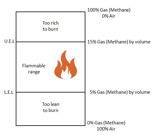Figure 1: Lower Explosive Limit (L.E.L) and Upper Explosive Limit (U.E.L)

The L.E.L is the critical point at which ignition or explosion occurs [11]. Once the L.E.L is reached, the danger of a fire or explosion is continuous all the way to U.E.L. For example the L.E.L of methane (CH₄) is 5% by volume and the U.E.L is 15% by volume. When a confined space reaches 2.5% of methane by volume this would be equal to 50% L.E.L which means that 5% methane by volume would be 100% L.E.L.  Between 5 to 15% by volume, a spark could cause an explosion. Different gases have different percentage by volume concentrations to reach 100% L.E.L.

2.3.  Toxic Atmosphere

The main toxic gases in confined space are carbon monoxide (CO) and hydrogen sulphide (H₂S) [4]. It may leak from products that are stored due to improper procedure or poor ventilation. The activities inside the area such as welding, painting, scraping and sanding may produce the toxic gases. The toxic fumes produced from nearby activities may flow and accumulate inside the area.

Workers expose to toxic gases in the atmosphere may be injured or killed by the gas. At certain concentrations, some toxic gases become too dangerous. At such levels, even a brief exposure can cause permanent health effects such as brain, heart and lung damage or the substance may render workers unconscious so that they cannot escape from the confined space. The Life-Threating Effects of carbon monoxide and hydrogen sulphide are listed in Table 2 and Table 3 respectively [11].

Table 2: Effect of carbon monoxide exposed period

Exposure (ppm)	Time	Effects and symptoms
35	8 hour	Permissible Exposure Level
200	3 hour	Slight headache, discomfort
400	2 hour	Headache, discomfort
600	1 hour	Headache, discomfort
1000 to 2000	2 hour	Confusion, discomfort
2000 to 2500	30 minutes	Unconsciousness
4000	> 1 hour	Fatal

Table 3: Effect of hydrogen sulphide exposed period

Exposure (ppm)	Time	Effects and symptoms
10	8 hour	Permissible exposure level
50 to 100	1 hour	Mild eye and respiratory irritation
200 to 300	1 hour	Marked eye and respiratory irritation
500 to 700	½ to 1 hour	Unconsciousness, fatal
> 1000	1 minutes	Unconsciousness, fatal

3. Fundamental of Electronic Nose System

3.1.  Electronic Nose

The e-nose as a device to mimic the discrimination of the mammalian olfactory system for smell is introduced in 1982 [12]. Initially the instrument used three different Metal Oxide Semiconductor (MOS) gas sensors to identify several chemical volatile compounds by using the response steady state signals. Then Gardner [13], described the e-nose development comprise of: (1) a matrix sensor to simulate the receptors of the human olfactory bulb, (2) a data processing unit that performs the same function as the olfactory bulb and (3) a pattern recognition system that would recognize the olfactory patterns of the substance being tested, which is a function performed by the brain in the human olfactory system. Figure 2 shows the similarity between human olfactory system and the e-nose system.

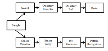Figure 2: Similarity between human olfactory system and e-nose system

3.2.  Sample Handling

The sample handling is a process to deliver the air sample to the sensor array. In the detection process, a sensor chamber is used to locate the sensor array where it interacts with the air sample. The data processing unit and pattern recognition algorithm will process the acquired data and classify them accordingly. The standard e-nose operating procedure includes determination of sample preparation and sampling method. The sample preparation procedure is determined by the type of sampling either static or dynamic method [14].

For static sampling, the sensor array and the sample is located at the same place in the chamber. The reading of sensor array is taken from the sample after the headspace in the chamber is homogenised. For dynamic sampling, the sensor array and the sample are at different or separate locations. The chamber is designed to locate a set of sensor arrays in one cavity and the sample is delivered into another cavity in order to be exposed to the sensors. This is also known as the Odour Capturing Module (OCM). The static sampling method is suitable to implement at a laboratory and not practical for outdoor use, while OCM is suitable to implement in both environments. However, the OCM must be purged to clean the chamber cavity after every sampling process to ensure sensor stability and repeatability for the next sampling process to produce consistent output readings [15].

Sample handling is a critical step affecting analysis by e-noses. The quality of the analysis can be greatly improved by adopting an appropriate sampling technique. To introduce the volatile compounds present in the headspace (HS) of the sample into the e-noses detection system, several sampling techniques have been used [16]. Various types of systems have been developed and are used to gather an air sample for analysis such an electric air pump which is used to suck the outside air sample into the sensor chamber [17]. A tube connected to a dedicated pump is generally used to direct the air sample into the e-nose. Other than that, the air sample delivery system was designed to provide seamless control over the operation by using a fan [18].

3.3.  Sensor Chamber

A sensor chamber is used to accommodate the sensor array’s interaction with the air sample. The chamber must be properly developed for optimum sensor response measurement. The design will emphasize optimum sensor response, stability, reproducibility and repeatability [19]. The air sample flow inside the chamber should be homogenous with low velocity to minimise the recirculating zones and stagnant volume [7]. This homogenous flow is to ensure that the sensor arrays are exposed simultaneously to the air sample for optimum response measurement. The sensors positions in the chamber can be either in a series or parallel to the air sample. The different sensors position from the chamber inlet will cause a time shift in each sensor response to the air sample. Since the distance between the sensors is small, so the time shift effect can be ignored [20].

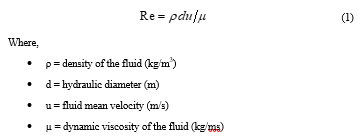
The symmetric structure will enable sensor arrays to respond simultaneously to the incoming air sample. However, this structure size is quite large to accommodate the sensor arrays in one area. The chamber development must focus on the structure geometry, material selection, type of flow and sensors position which will optimise its performance.  The geometry of the chamber should be symmetrical to enable the air sample to be exposed to the sensor arrays efficiently. The flow of air sample is usually characterized using dimensionless ratio known as Reynolds number (Re). The Re is a measure of the kinetic forces to the viscous forces in a flowing fluid. The Navier-Stokes formula shown in Equation 1 is used to solve for air sample flow characteristics [21].

3.4.  Gas Sensor

The gas sensor is used by the e-nose to interact with the air sample inside the sensor chamber. The interaction will cause a change in certain chemical and physical properties known as sensor responses that will convert into electrical signal. These sensor responses will be acquired by a laptop computer that links wirelessly with the e-nose to be used by an off-line signal processing method. The instrument sensors sensitivity should be suitable with the application’s volatile compounds [12]. The sensors are also selected based on their characteristics which include fast response, stability, reproducibility and reversibility.

The principles of gas sensors are optical, thermal, electrochemical and gravimetric [22]. Most e-nose devices use electrochemical sensors to detect chemical substances to response. The operating principles are based on changes in the conductivity of sensing material by either adsorption or absorption of the gaseous molecules. The sensor conductivity depends on the material used and is relative to the sample concentration. The gas sensors performance is measured by several criteria and their behaviour include sensitivity, selectivity, stability, detection limit, responses time, recovery time, life cycle and operating temperature [23]. All these criteria are very important to take into consideration during the selection of the gas sensors. The MOS gas sensor was widely use selected based on its stable response in performance.

3.5.  Microcontroller System

The e-nose normally uses an embedded controller which is a microcontroller with embedded software for operation, data acquisition and classification [24]. The control and system software is embedded in the instrument memory that may perform concurrently during operation. A microcontroller is a component that is used to control the sampling process for acquiring the sensor response signals to be processed by a personal or laptop computer [25]. The microcontroller has good processing capabilities and a flexible interface to the instrument’s components which make it the ideal choice as the controller. The microcontroller memories are RAM, Flash ROM and EEPROM. The Flash ROM memory is where the program is stored, also called program memory. RAM is used for the temporary data during run-time. The EEPROM is used for data memory that needs to be retained during power failure. This microcontroller memories ability makes it suitable for e-nose operation that consist multimodal sensor to send the signals concurrently.

      Currently, the dsPIC33 microcontroller type from Microchip Technology Inc. as the embedded controller was used in e-nose system development [26]. The microcontroller was designed using Surface Mounted Technology (SMT) component to improve the performance by reducing the signal to noise ratio (SNR). The microcontroller also converts the acquired analogue signal to digital by using an on-board Analogue-to-Digital Converter (ADC).

3.6.  Signal Conditioning

      The e-nose signal conditioning frame work as shown in Figure 3 consists of an interface circuit, conditioning circuit and filter [27]. The interface circuit measures the sensor responses and converts it into output voltage that varies with conductive change in the sensing element [28].  A conditioning circuit is used to buffer and amplify the signal to suit the microcontroller requirement. A voltage follower is used as a buffer to isolate the signal and as impedance matching of the sensors output. The noise is removed from the signal by using a passive Low Pass Filter (LPF) because it is good for removing a small amount of high frequency noise (>2 kHz).

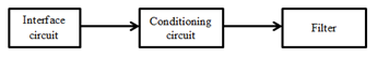Figure 3: The signal conditioning frame work

3.7.  Data Processing

      The e-nose will produce a time-series sensor response corresponding to the air sample. The sensor response as data also depends on ambient air, temperature and humidity. The process consists of pre-processing, dimension reduction, pattern recognition and results as shown in Figure 4.

Figure 4: Electronic nose data processing block diagram

      The chemo-metric processing technique that relates mathematical and statistical is used to extract the relevant information from the data [29]. This method uses multivariate analysis to discriminate the data simultaneously. The process uses either a statistical or biological classification method approach to classify or cluster the data qualitatively or quasi quantitatively. The analysis methods are divided into parametric, non-parametric, supervised and unsupervised [30]. A parametric pattern is when the data are Gaussian and the distribution feature is normal. Supervised method develops a classification model using known data while unsupervised method uses unknown data for the development.

3.8.  Pre-processing

      The e-nose raw data is highly susceptible to noise, uncertain value, and inconsistency pattern. The quality of the data affects the classification model result. The data needs to be pre-processed to improve its quality which will in turn improve the classification process [31]. The process is critical for data processing that involves preparation and transformation of the initial raw data.

3.9.  Feature Selection

      The e-nose time series acquired data consists of dynamic or transient and steady state sensor response [32]. Figure 5 shows the transient and steady state sensor response. Feature selection is used to select a certain region of the sensor response that contains relevant sample information. Most of the e-noses extract the steady state region from the sensor response for the pattern recognition process.

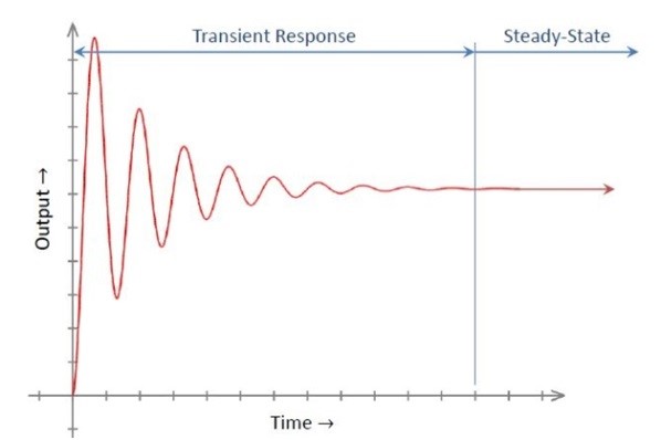Figure 5: The transient and steady state sensor response

3.10. Baseline Manipulation

      The baseline manipulation is a method that is based on the difference of the sensor response value between reference and sample [33]. The reference normally is the ambient air or nitrogen gas. Four baseline manipulation methods are commonly employed which are difference, relative, fractional and logarithm. The difference method is a widely used by directly subtracts the baseline and can be used to eliminate additive drift from the sensor response. Relative manipulation divides by the baseline, removing multiplicative drift and generating a dimensionless response. Fractional manipulation subtracts and divides by the baseline, generating dimensionless and normalized responses. The advantages of these processes will enhance the quality of data which contains the relevant sample information.

3.11. Normality Test

      The procedure in assessing a sample of data has a normal distribution are graphical methods (histogram, boxplots and Q-plots), numerical methods (skewness and kurtosis indeces) and normality test [34].  A normality test is a statistical process used to determine if a sample or any group of data fits a normal distribution or not to determine suitable types of data analysis.

      A normality test can be performed mathematically for example the Shapiro-Wilk (SW), Kolmogorov- Smirnov (KS) or Anderson-Darling (AD) test [34]. The power of test method proportionally increased with sample size and level but was still low for a small sample. The Kolmogorov- Smirnov test is the best with high sensitivity in rejecting null hypothesis [35]. The Shapiro-Wilk is suggested being to be used for a normality test, but Kolmogorov- Smirnov is popular [36].

      Basically the data skewness and outlier’s features indicate non-normality distribution. The data non-normality distribution needs to be transforming in order to process using the parametric classification method [35]. But the alteration on the original non-normality data will create curvilinear relationships that will complicate the interpretation. The data should us a non-parametric classification method when the distribution is not normal.

3.12. Multivariate Statistical Analysis

      The Multivariate Statistical Analysis is used to discriminate and classifier sample. It build discriminate and classifier models. Some of the multivariate analysis techniques are Principal Component Analysis (PCA) for discriminate and Support Vector Machine (SVM) for classifier. This technique is described in the following sub section.

3.13. Principal Component Analysis

The PCA is a dimension-reduction tool that can be used to reduce a large set of variables to a small set that still contains most of the information in the large set. The PCA will transform the number of original data with correlated variables (number of sensors) into uncorrelated variables (Principal Components, PC) and loadings or weight of each original variable of variance percentage.

Traditionally, PCA is performed on a square symmetric matrix. It can be a pure sum of squares and cross product (SSCP) matrix, covariance matrix (scaled sums of squares and cross products) or correlation matrix (sums of squares and cross products from standardized data). The SSCP and covariance do not differ, since these objects only differ in a global scaling factor. A correlation matrix is used if the variances of individual variants differ much or if the units of measurement of the individual variants differ. Basically, PCA can be represented in five steps [37]:

1. Normalize the data by subtracting the mean
2. Calculate the covariance matrix

iii.     Calculate the eigenvectors and eigenvalues of the covariance matrix

1. Choose components and form a feature vector
2. Derive the new data set

      The PCA result is shown by a two-dimensional (2D) or three-dimensional (3D) graphical plot that contains the original data’s important information and shows the PC percentage and group cluster which is being analysed visually. The PCA is used as the dimension reduction technique as it is the most widely used in e-nose data analysis.

3.14. Support Vector Machine

The SVM is a supervised learning model that is based on statistical learning theory for data classification and regression [38]. The SVM training used data with known class when designing a linear classifier hyper plane model for separate group. SVM is targeting clear maximum margins between the hyper plane and closest training. In addition, the SVM optimized classification decision function is based on structural risk minimization in order to avoid over fitting.

In more complicated for non-linear cases, SVMs employ the kernel trick where a positive definite kernel function is used to map the input data into a high dimensional transformed feature space and this method regularly used by the e-nose community that used multisensory system [39]. The SVM mathematical modelling and algorithm can be referring in [40]. Although SVMs were initially developed for solving two-class problems, but it is also can be easily adapted to tackle multiclass problems. The two common techniques consist of:

1. One per class (OPC). This method is also known as “one against others”. OPC is simple and results in reasonable performance. K SVM classifiers are trained, each of which separates one class from the other (K−1) classes. For each measurement, x, to be classified, K SVM decision outputs fk(x), 1 ≤ k ≤ K are obtained. The class of measurement x, j, is determined as fj(x)/fk(x) > 1 for (1 ≤ k ≤ K) / = j.
2. Pairwise coupling (PWC). This method is also known as “one against one”. This method trains (1/2)K(K−1) binary SVM classifiers. To classify a measurement, PWC combines the scores of these (1/2)K(K−1) classifiers. Each of the (1/2)K(K−1) binary SVM classifiers provides a partial decision for classifying a measurement. There are different methods of combining the obtained classifier and the most common is a simple voting scheme. When classifying a new instance each one of the base classifiers casts a vote for one of the two classes used in its training.

Since SVM does not require any estimation of statistical distributions of classes to accomplish the classification task, the application is widely used in many fields. For examples, the classifier performance is excellent in determination of green tea quality grades [41] and identification of selected features on Mexican coffee [42].

3.15. Artificial Neural Network

      The non-linear e-nose sensor responses have to be converted to linear before they are classified using linear classifier methods. However, high volume of data from complex instrument’s sensor responses is difficult to produce an efficient classification model.  The Artificial Neural Network (ANN) has good learning, generalization and noise tolerance that is suitable for the e-nose non-linear data [43]. It has the ability to learn the complex interaction between the array of sensors and the air sample [44]. The network’s ability to compensate the moderately sensitive sensors towards the air sample has improved the classification success rate.

      The ANN is a mathematic model in which the nodes are interconnected with each other with weights and biases to form the network architecture. The architecture depends on the mathematical analysis of task criteria. The common network structure uses fully connected three-layer architecture models which are made of input, hidden and output nodes. Figure 6 shows that an ANN model consists of the input layer, hidden layer and output layer.

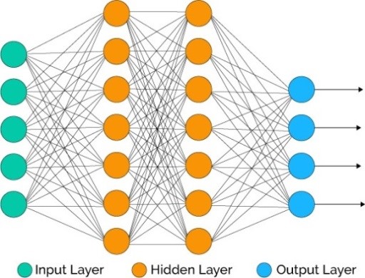Figure 6: Basic neuron model showing the components and connections

Each neuron has a few weighted inputs and finally generates one output. The output is a function on these weighted inputs. Various types of functions can be used to calculate the output in a neuron. One type of neuron is called a perceptron which takes a vector of real-valued inputs and calculates a linear combination of these inputs. It outputs 1 if the result is greater than some threshold and -1 otherwise. Given inputs x₁…x_n, this perceptron function is shown in Equation 2 till Equation 5:

      A sigmoid unit is equal to a perceptron. Firstly, it calculates the linear combination of its inputs and then applies a threshold to the result. However, this threshold is continuous comparing with a perceptron with a discontinuous threshold. The output of sigmoid function is between 0 and 1 (or between -1 and 1) and increases monotonically with its inputs. The sigmoid unit maps a very large input domain (-∞,∞) onto a small range of outputs (0,1) or (-1,1).

      A particular transfer function is chosen to satisfy some specification of the problem that the model is attempting to solve [45]. During training, the model learns from the input neuron and gradually adjusts its weight to reflect the desire outputs [46]. The network model is tested by using the randomised unused testing data. The process uses the unknown data to test the network’s generalisation ability of the classification model. The performance of the network model is given by the Equation 6.

      Types of ANNs refer to the model learning methods: supervised, unsupervised and reinforcement. These include Multilayer Feed-Forward Perceptron (MLP), Fuzzy ARTmaps, Kohonen’s Self-Organizing Maps (SOMs), Probabilistic Neural Network (PNN) and Radial Basis Function Neural Network (RBFNN). The MLP, PNN and RBFNN are supervised types of classifiers that are normally used for e-nose applications [47]. The classification results using RBFNN is the most stable with a high classification success rate [48].

3.16. Radial Basis Function Neural Network

The RBFNN consists of three layers includes input layer, hidden layer and output layer. The method approximation capabilities are based on the superposition of local models of the response system. The output layer only computes a linear combination of the activation of the neurons in the hidden layer. The input output multivariate relationship is given by using Equation 7 and also can be written in matrix form in [49]:

Where,

• y_ij is i,j-th element of the output matrix Y_N,K
• N is the number of observations (data)
• K is the number of outputs in the RBFNN (or responses)
• If denote M as the number of hidden neurons (or the RBF canter’s), w_mj is m,j-th element of the weight matrix W_M+1,K, m = 1, 2, …, M
• M+1 is the number of hidden neurons add bias (b)
• X_NM is the input patterns
• c_m is the square centroids matrix M x M
• E_NK is the matrix of residuals of e_ij
• Y_NK(x)=d_ij is the process output

           The activation of every neuron depends on the distance of the input vector to the prototype represented by the radial basis function and neuron parameter. The radial activation function network provides a nonlinear method of interpolating between numbers of different areas, time-series estimation and classification. The method always converges at the same point when trained with the orthogonal least squares algorithm. The advantage of the classifier is that the network has no local minima problem [50].

4. Electronic Nose Development

4.1.  System Structure

The e-nose system structure includes the sensing module, signal conditioning, microcontroller and embedded software. The instrument peripherals (i.e. an air pump, keypad, graphical Liquid Crystal Display (LCD), purging system, power supply and wireless Radio Frequency (RF) communication are controlled by the microcontroller) as shown by Figure 7.

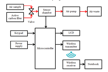Figure 7: The e-nose block diagram

4.2.  Sensing Module

The sensing module consists of sensor arrays for gas detection and a sensor chamber to locate the sensor arrays. Each gas sensor should have a different sensitivity profile over a range of hazardous gases for the confined space application. The process had selected suitable sensors with varying sensitivity to generate the responses known as smell prints. The process had reduced the instrument size, cost of the sensors, power consumption and will increase classification performance.

The gas sensors performance is measured by several criteria such as sensitivity, selectivity, stability, detection limit, response time, recovery time, life cycle and operating temperature [23]. All these criteria are very important to consider during selection of the gas sensors. The developed e-nose sensing module used four selected MOS gas sensors that are normally and widely used for environmental monitoring [51]. The sensors were selected based on each sensor varying sensitivity and selectivity that generated a smell print profile corresponding to the air sample. The selections were based on the confined space main hazardous gases effective value with different sensitivity manufactured by Figaro Inc. and Synkera Technologies Inc. as listed in Table 4. The sensors are able to detect main hazardous gases effective value to effect human for oxygen at between 0-30%, carbon monoxide at 35 ppm, hydrogen sulphide at 20 ppm and methane 5%. For monitoring the environmental conditions, the temperature and humidity sensor (SHT75) from Sensirion company was also located under the developed instrument due to its characteristics and ability (refer to appendix A). The sensor uses two wires through Serial Peripheral Interface (SPI) communication to communicate with the embedded controller.

Table 4: E-nose sensors selection

Category	Target Parameter	Sensor	Sensitivity (ppm)	Sensitivity (%)	Operating Temperature (°C)
Oxygen	Oxygen	Sk-25F	–	0 to 30	-10 to 50
Toxic	Carbon Monoxide	TGS 2442	30 to 1000	–	-10 to 50
	Hydrogen Sulphide	PN 714	1 to 100	–	-10 to 50
Flammable	Methane	TGS 2612	–	1 to 25	-10 to 40

The e-nose sensor chamber was designed and simulated using Computational Fluid Dynamic (CFD) SolidWorks version 2012 software. The SolidWorks software was used to create the Three Dimensional (3D) model of the chamber structure. Then the CFD was used to simulate and analyze for optimum air sample flow inside the chamber cavity to expose to the sensors. The analysis was based on the pressure, velocity and Reynolds (Re) number that were generated during the simulation.

The simulation finding was used to enhance the sample flow optimization, structure geometry, material and reduce the chamber dead zone [52]. The geometry should be symmetrical for efficient sample flow inside the chamber cavity. The simulation analyzed the best sensor position between series and parallel chamber design for optimum sample flow exposure to the sensor array and the series type was chosen shown in Figure 8.

Figure 8: (a) Isometric and (b) explode view for chamber design

4.3.  Signal Conditioning Board

      The e-nose MOS gas sensors were attached to the signal conditioning board. The board is used to enhance the sensor responses signal suitable for the data acquisition by the microcontroller. The unit consists of the interface circuit, amplifier, filter and Analogue-to-Digital Converter (ADC) as shown in Figure 9.

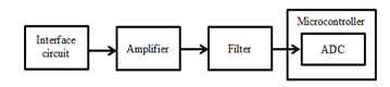Figure 9: The signal conditioning block diagram

      The interface circuit will measure the sensor responses and convert it into a constant current circuit. The sensor heater was used to increase the sensor temperature to around 300^oC and the heater circuit is including in the sensor.  The sensor response was calculated by using Equation 8.

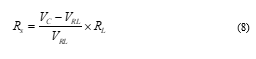Where,

• R_s is the sensor resistance or responses
• V_c or V_cc is the circuit voltage
• V_RL is the voltage load resistor or voltage output (V_out)
• R_L is the load resistor

The R_L value used to limit the sensor output voltage and V_RL up to five volts. The R_L were using 10 KΩ with 1% accuracy to enable the output voltage range suitable for the microcontroller. The signals from sensors are in analogue form and voltage divider rule are applied to the signal conditioning circuit. The sensor principle is impedance with low range (refer to appendix A) and the MCP602 Integrated Circuits (IC) unity gain voltage follower from Microchip Technology Inc. was used as the signal amplifier. The amplifiers high input and low output with good impedance matching will minimise the loading effects to the microcontroller ADC.

      A passive Low Pass Filter (LPF) was used to filter the sensor responses signal from unwanted noise. The passive filter was used because of its fewer components and low noise as compared to active filter. The cut off frequency was calculated by Equation 9. The LPF was designed to allow frequencies below 2 KHz to pass, while blocking frequencies above it.

Where,

• fc is the cut off frequency
• R is the resistor value
• C is the capacitor value

Two signal conditioning circuit boards were designed and developed for sensors located at the left and right of the sensor chamber. The circuit boards were designed using Power Logic software. Then it was converted into a schematic diagram for the board etching process by using Power PCB software. Then both signal conditioning board is etching for components placement through soldering process. The developed sensing module includes sensor chamber and signal conditioning board. The left side board is for carbon monoxide and methane while oxygen and hydrogen sulphide sensors are on the right.

4.4.  Controller Board

      The controller Printed Circuit Board (PCB) was also designed using Power Logic and Power PCB software. The fabrication is as shown in Figure 10. The PCB main component uses Surface Mount Technology (SMT). The electronic components were laid out on a two-layer plated through hole PCB. All the ICs were decoupled to ground with capacitors to reduce noise from the circuits. The ground plane tracks at the bottom layer were kept to a minimum to reduce the signal to Noise Ratio (SNR). The acquired data is transmitting through Zigbee wireless Radio Frequency (RF) communication.

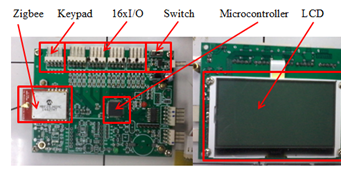Figure 10: The controller board front and back view

4.5.  Microcontroller

The e-nose system controls and data processing use the microcontroller with embedded software. The dsPIC33 microcontroller from Microchip Technology Inc. was selected because its 40 MIPS is good for high processing speed and its 16-bit data bus is suitable for the instrument operation in real time. The microprocessor flash memory is 256 KB and 30 KB for RAM are large enough and capable of handling the data acquisition operation and system control at the same time.

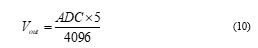
      Furthermore, the dsPIC33’s built-in 12-bit ADC conversion speed is capable of simultaneously sampling from all the analogue sensor responses signal. The digitized data is stored inside the microcontroller flash memory and sent to laptop computer which is linked through Zigbee wireless RF communication during the data acquisition process. The output digital signals are expressed in numbers ranging from 0 to 4095 and sensors voltage output is calculated by Equation 10.

4.6.  Wireless Communication

The e-nose wireless communication was developed using Zigbee (MRF24J40MC) module from Microchip Technology Inc. based on 2.4 Gigahertz (GHz) IEEE Std. 802.15.4™. This module has been chosen as a medium for communication because its communication range can reach up to 4000 feet and the temperature range is at -40 ° C to + 85 ° C which are suitable for confined space applications. It is also popular because its miniature size, simple circuit and low power. The Zigbee module has a 50Ω Ultra Miniature Coaxial (U.FL) connector to connect to an external 2.4 GHz antenna. The module interfaces to the microcontrollers through a four wire Serial Peripheral interface (SPI), interrupt, wake, reset, power and ground as shown in Figure 11.

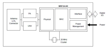Figure 11: Wireless Zigbee (MRF24J40MC) module block diagram

4.7.  Input and Output Devices

The e-nose main controller board was interfaced with a four-button keypad as the input device. The input is used as the user interface to select the instrument program menu. A 128×64 character graphic Liquid Crystal Display (LCD) from Topway Displays brand was selected as the instrument display unit (output). The LCD is used to display several instrument attributes such as operation, data acquisition and utilities.

4.8.  Purging System

The sampling system will deliver the air sample to flow into the sensor chamber. The system is essential to ensure that all sensors are exposed to the air sample effectively during the sniff cycle. For this confined space application the e-nose has a self-purging function to ensure that the sensor chamber is purged accordingly [1].

Figure 12 shows a pneumatic system that has been designed as the e-nose self-purging system. The system has a 3-way solenoid electro-valve that was placed between instrument inlet and sensor chamber. During sniff cycle the electro-valve would allow the air sample from the confined space atmosphere to flow into the sensor chamber through channel one. While during purging cycle, the electro-valve would allow filtered air through the carbon filter to purge the sensor chamber cavity through channel two. The system is programmed and controlled by the instrument’s microcontroller.

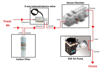Figure 12: The e-nose purging system

4.9.  Power Unit

      The e-nose system uses a single 12 volt lead acid battery as the power supply. The power supply is used for the air pumps, electro-valve, signal conditioning boards and main controller board. The PCB consists of two unit voltage regulators (LM2575) used to provide 5 volts of power for the sensor measuring circuits, amplifiers, analogue multiplexer and relay.

4.10. Enclosure

      The enclosure or casing for the e-nose was selected based on space for component placement and the material used. The plastic enclosure was used because of its non-flammable properties when exposed to high temperatures. It also did not interfere with data acquisition during the sniff operation. Figure 13 shows the enclosure with dimension of 22cm (L) x 30cm (W) x 14cm (H) and the instrument’s complete hardware development.

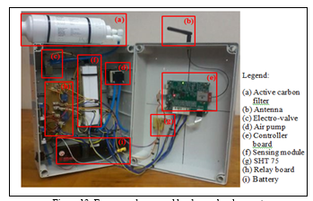Figure 13: E-nose enclosure and hardware development

4.11. Software Development

      The e-nose embedded software is used to integrate hardware to enable the instrument operate as a system. The acquired data transferred wirelessly from the instrument to a laptop computer that is received and displayed through Graphical User Interface (GUI). The data is processed and classified using an off-line method by utilizing MATLAB software.

4.12. Embedded Control Software

      The e-nose embedded software has been developed on the laptop computer using dsPIC33 C compiler version 8.0 from Microchip Technology Inc. The compiler was bundled inside the MPLAB Integrated Development Environment (IDE). The menu driven program contains the instrument control, data acquisition, communication and utilities.

4.13. Graphical User Interface

      A Graphic User Interface (GUI) was developed using Visual Basic 6.0 (VB6) software on a windows 7 platform. The GUI is used for receiving and recording the sensors output digital signal that is transmitted wirelessly by the e-nose to laptop computer. The GUI will display the sensor digital output signal that is plotted in a single bar graph according to their concentrations as shown in Figure 14. The instrument sensor digital output signals that are displayed by the GUI in real time are saved as a text file.

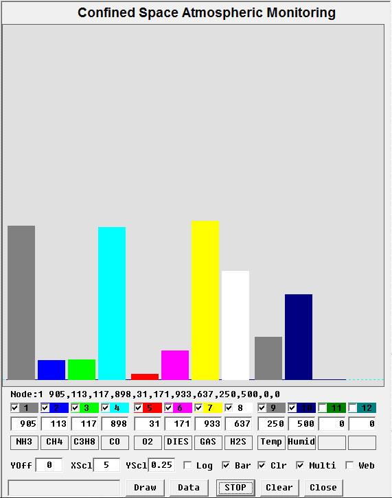Figure 14: Graphic User Interface (GUI) for sensor responses

4.14. Converting ADC Data to parts per million

      The developed GUI is also able to convert the e-nose sensor digital output signal as data in ADC value to parts per million (ppm) and percentage correspond to the air sample concentration. Based on the e-nose MOS gas sensors data sheet, the MOS gas sensors have a linear correlation between the sensor responses and air sample concentration. The sensor response gradient (m) and constant value (k) that intersect at x = 1 was calculated using Equation 11 and Equation 12.

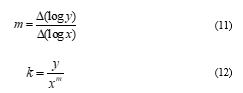Where,

• m is the gradient
• y is the sensors response (Ω) value
• x is the sample concentrations (ppm) value
• k is the intersection point at axis x=1

      Based on the calculated value of the sensor response gradient and constant value, the sensor digital output signal in ppm value, x can be calculated by using Equation 13.

      For the flammable gas (i.e. methane), the sensor digital output signal is measure in percentages by using Equation 14. The developed GUI for the instrument sensors digital output signal conversion is shown in Figure 15.

Where,

• x_% is the sample concentrations in percentage
• x_ppm is the sample concentrations in ppm

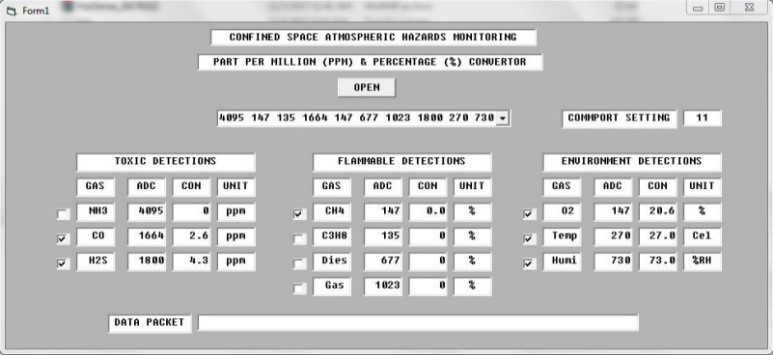Figure 15: Graphic User Interface (GUI) for data conversion

5. Experimental Setup

      The e-nose was tested in laboratory and field environments. This process will ensure the instrument functionality, performance and reliability were satisfied. The first experiment was conducted to test the performance of the purging system. After that, the instrument was calibrated to test its response to various air sample concentrations.  Lastly the instrument was tested in a hospital confined space (i.e. mechanical room) for field atmospheric hazards monitoring.

5.1.  System Setup

      Dynamic headspace technique was used for the e-nose sampling process. The instrument system setup was set according to the parameters listed in Table 5.

Table 5: The e-nose system setup parameter

Operation	Time (s)	Air pump	Electro-valve
Switch on e-nose and run GUI	30	OFF	OFF
Sensors pre-heat period	90	OFF	OFF
Purge cycle	60	ON	ON
Holding period after purge cycle	30	OFF	OFF
Sniff cycle	30	ON	OFF
Holding period after sniff cycle for data acquisition	200	OFF	OFF

Based on the system setup parameters, the e-nose uses the dynamic headspace sampling method includes “purge”, “sniff” and “hold”. The method will hold the air sample in sensor chamber to enhance the e-nose sensitivity. The setup parameter values were based on the selected sensors characteristics. The data acquisition experiment procedures are as follows:-

1. Switch on the e-nose and run the GUI on a laptop computer to test the communication.
2. Pre-heat the instrument sensors to ensure the MOS gas sensors reach the optimum operation temperature.

• Activate the self-purging procedure (purge cycle) by activating the 3-way solenoid electro-valve channel two. This would allow the ambient air to flow through the active carbon filter by using the air pump. The clear reference air will flow into the sensor chamber and flush out the previous air sample. Then the instrument will remain idle for about 30 seconds to allow sensors response to return to its basic value.

1. Sniff cycle, the 3-way solenoid electro-valve channel one is activated for the instrument expose to the air sample. The headspace air sample will flow into the sensor chamber by using the same air pump.
2. The air sample will be held in chamber for 200 seconds that will expose the sensors for optimum interaction and sensor response reach steady state.
3. The steady state sensor response data is transfer wirelessly through the Zigbee module to a laptop computer that is displayed and saved by the GUI. The GUI will record 200 data at one data per second baud rate based on the sensor’s response.

vii.       Repeat steps (iii) to (vi) for another nine times that will generate 2000 data which is used for the data processing.

5.2.  Purging Testing

The e-nose self-purging test experiment was conducted at the biomaterials laboratory, School of Mechatronics Engineering, Universiti Malaysia Perlis (UniMAP). The laboratory temperature was 25°C with 75% Relative Humidity. The room temperature and humidity was continually observed and recorded.

The experiment sampling process used the instrument system setup as explained in section 5.1. This experiment was conducted to test its ability to flush out the air sample from the sensor chamber enabling gas sensor responses return to its basic value. The experiment had to follow the data acquisition procedure.

      Initially the instrument purge cycle operation experiments were activated using laboratory ambient air as the reference. Then the instrument purge cycle was repeated by using the self-purging system which is activated by the three-way solenoid electro-valve channel two. This allows the ambient air to flow through the active carbon filter. The reference air will flow into the sensor chamber and enables sensors response to return to their basic value. Both purging method sensor responses are analyzed for their performance.

5.3.  System Calibration and Validation

E-nose calibration and validation experiments were conducted also at the same laboratory. The laboratory temperature was 25°C with 75% Relative Humidity. The room temperature and humidity was continually observed and recorded.

The experiments were conducted in laboratory in a fume hood because it will absorb any leaking of the hazardous gases as shown in Figure 16. The e-nose sampling process involves two gas sampled cylinders with different concentration as listed in Table 6. The experiment sampling process used the e-nose system setup as explained in section 5.1. The experiment had to follow the data acquisition procedure.

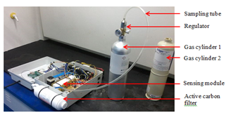Figure 16: The e-nose calibration and validation testing

Table 6: The component and concentrations for gas cylinder one and gas cylinder two

Components	Concentrations
	Cylinder 1	Cylinder 2
Hydrogen sulphide (H2S)	10 ppm	< 1 ppm
Carbon monoxide (CO)	50 ppm
Methane (CH4)	2.5 %
Oxygen (O2)	18.0 %	20.8%

The gas in cylinder one which contains oxygen, hydrogen sulphide, carbon monoxide and methane used for the calibration while cylinder two which contains air with zero grades (<1 ppm) were used for the validation.

      Initially, the experiments were conducted by using gas from cylinder one (a mixing of hydrogen sulphide, carbon monoxide, methane and oxygen) as the sample to identify and calculate the calibration value. Then the experiments were repeated by using gas cylinder two which contain air with zero grades. The experiments were used to verify the e-nose ability to responses with lowest concentration of air sample.

      E-nose performance was validated with an Altair 5X Multi Gas Detector from MSA brand which is able to detect hydrogen sulphide, carbon monoxide, methane and oxygen [53]. The instrument temperature and humidity measurement value were also validated by using the Humidity Alert Detector from Extech as shown in Figure 17.

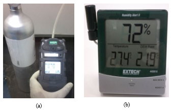Figure 17: (a) Altair 5X Multi Gas Detector and (b) Humidity Alert detector

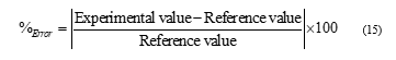
      Initially both gas cylinders were used as air samples for the gas detector. The validate instrument measurement was used as the reference value. Then the experiments were conducted for the instrument using both gas cylinders. The different measurement values between the instrument and validate instrument which are known as percentage error (%_error) by using Equation 15 were adjusted to be less than 10% by modifying the embedded instrument data acquisition program [53]. The experiments were repeated to 10 times for the instrument and validate instrument using both gas cylinders for validation process.

Where,

• %_Error is percentage error value
• Experimental value is e-nose sensor responses data
• Reference value is validate instruments data

      E-nose temperature and humidity measurement values were also compared with the commercial temperature and humidity meter. The different measurement values were also adjusted to less than 10% by modifying the embedded instrument data acquisition program. The experiments were also repeated for the instrument to validate the temperature and humidity measurements values.

5.4.  Field Environment Testing

E-nose field environment experiment was conducted in a confined space (i.e. mechanical room) at the Hospital Sultanah Bahiyah, Alor Setar, Kedah. There are two set generators placed in the mechanical room to generate electricity when electricity is suddenly cut off in the hospital building. This room is potentially exposed to the atmospheric hazards when there is a leak at the generator that uses diesel fuel to operate. During the operation, the carbon monoxide gas will release and oxygen level became limit because eliminate by this gas.

This mechanical room is also chosen because of its appropriate area and the distance that allows wireless communication devices to function fully without losing any data. The room size was 20m (L) x 10m (W) x 5m (H) and the room average temperature was 31°C with 63% Relative Humidity. This room temperature and humidity condition has no effect to the sensors ability in term of drift response and sensitivity changes after calibration experiment testing were done based on the sensors operating temperature. The room temperature and humidity were continually observed and recorded.

Four locations, ambient (outside room), location one, location two and location three were selected for data acquisition. The purpose of these locations was to prove the ability of the instrument to be able to classify the concentration of gas according to their location. The experiment started with data acquisition at outside room as reference air, followed by location one, two and lastly at location three. The generator and data acquisition location in the mechanical room are illustrated in Figure 18. The experiment sampling process used the e-nose system setup as explained in section 5.1.

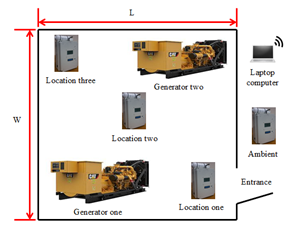Figure 18: Data acquisition locations in mechanical room

6. Results and Discussion

6.1.  Purging Testing

      This section discusses the data analysis for the purging testing to compare reading between normal ambient air and the filtered ambient air. The analysis utilised the statistical multivariate technique to discriminate between two different samples.

      E-nose sensor responses were a time series waveforms profile. The sensor responses purging cycle using laboratory ambient air and ambient air through an active carbon filter are shown in Figure 19 and Figure 20 respectively. The reference air flows into the sensor chamber and enables the sensor responses to return to their basic values.

The average for 10 times readings from sensor responses between the ambient air and filtered ambient air are listed in Table 7. The readings show that sensor responses for the ambient air through the active carbon filter is lower than ambient air without filter. This means that the active carbon filter is able to flush out the air sample from the sensor chamber better to enabling gas sensor responses return to its basic value and become stabilized during purge cycle.

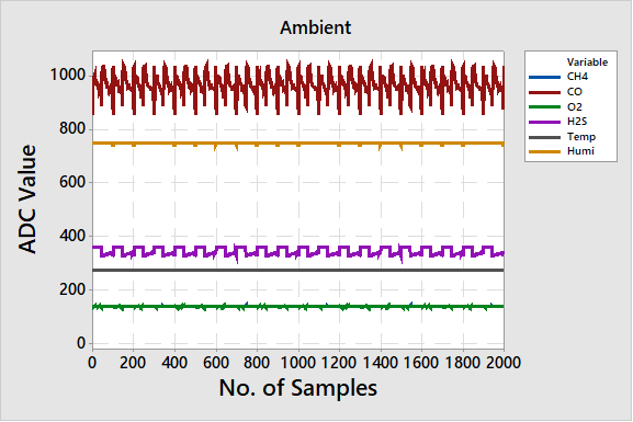Figure 19: Sensor responses for ambient air

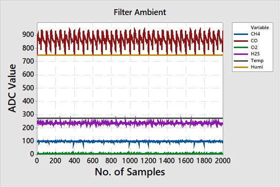Figure 20: Sensor responses for ambient air through active carbon filter

Table 7: Average sensor responses for purging testing

Parameter	Methane (ADC value)	Carbon monoxide (ADC value)	Oxygen  (ADC value)	Hydrogen sulphide (ADC value)
Ambient air	150	950	140	350
Active carbon filter	100	850	10	250

The PCA used the correlation matrix method because for all samples, the sensor responses data variances were completely different so the data variances were standardized. Figure 21 shows the PCA score plot for instrument purging testing.

      Consists of six total principal component’s (PC) that represent number of instrument sensors and a 2D-PCA score plot was used because the first two PC variation accounted for 99.43% (PC1 was 91.21% and PC2 was 8.22%) of the total data more than 90% which contain useful information [54]. The plot shows that data for ambient air and ambient air through an active carbon filter are successfully discriminate into two groups. This shows that the proposed self-purging system capability is successful in providing reference air for the instrument purge cycle operation.

6.2.  Calibration and Validation

      This section discusses the data analysis for the calibration process by calculating the calibration value. The validation between developed instrument and validated instrument is to verify its detection performance and reliability.

      Sensor responses for the e-nose calibration which used gas cylinder one and gas cylinder two are shown in Figure 22 and Figure 23. The plotted graph shows that the different detection reading between both gas cylinders. The feature selection process was applied to the raw data and 100 steady state responses were select for both gas cylinders detection.

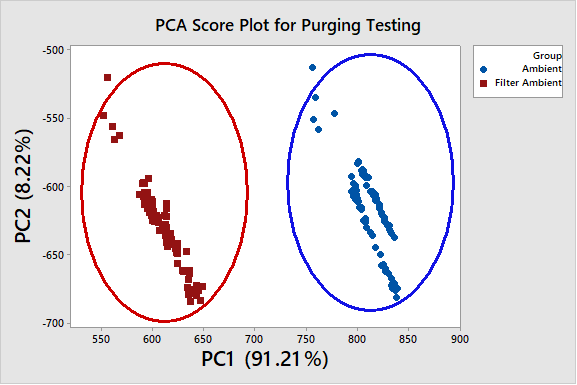Figure 21: PCA score plot for purging testing

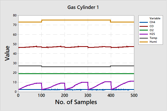Figure 22: Sensor responses for gas exposure from cylinder one

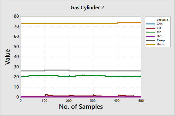Figure 23: Sensor responses for gas exposure from cylinder two

      The calibration value is the different reading between the e-nose average sniff and the commercial detector as a validated instrument. The percentage error (%_Error) calculation for instrument sensors when exposed to the concentrations of gas cylinder one is shown in Table 8. The instrument sniff reading was 2.03% for methane, 46.83 ppm for carbon monoxide, 18.68% for oxygen, 6.68 ppm for hydrogen sulphide, 26.40°C for temperature and 74.20% Relative Humidity for humidity sensors. The different values between instrument sniff and validate instrument shown by the methane is 0.47%, carbon monoxide is 3.17 ppm, oxygen is 0.12%, hydrogen sulphide is 3.32 ppm, temperature is 0.40°C and humidity is 0.20% Relative Humidity.

      Results from these different values are used as the calibration values for each sensor when performing the next detections. The percentage error was than calculated and it shows 18.80% for methane, 6.34% for carbon monoxide, 0.63% for oxygen, 33.20% for hydrogen sulphide, 1.53% for temperature and 0.27% for humidity sensors.

Table 8: Calibration value and percentage error calculation before calibration

	Methane (%)	Carbon Monoxide (ppm)	Oxygen (%)	Hydrogen Sulphide (ppm)	Temperature (°C)	Humidity (%RH)
E-nose sniff	2.03 ±0.08	46.83 ±0.12	18.68 ±0.02	6.68 ±0.93	26.40 ±0.36	74.20 ±0.24
Altair 5x	2.50	50.00	18.80	10.00	–	–
Humidity Alert	–	–	–	–	26.00	74.00
Calibration value	0.47	3.17	0.12	3.32	0.40	0.20
Percentage error (%)	18.80	6.34	0.63	33.20	1.53	0.27

      The same sampling method process is performed, but this time by adding the calibration value for the instrument sensors when exposing them to the concentrations of gas in cylinder one. The result is shown in Table 9. The different readings between instrument sniff and validate instrument shown by the methane is 0.04%, carbon monoxide is 1.18 ppm, oxygen is 0.24%, hydrogen sulphide is 0.50 ppm, temperature is 0.60°C and humidity is 0.40% Relative Humidity. The percentage error was then calculated and it shows 1.60% for methane, 0.36% for carbon monoxide, 0.21% for oxygen, 5.00% for hydrogen sulphide, 2.22% for temperature and 0.80% for humidity sensors. Since the percentage error is decreased to less than 5.00% which is within the standard total difference allowed (less than 10%), the results were considered as valid and acceptable [55]. This proved that the instrument is trusted and ready for real field environment testing.

Table 9: Calibration value and percentage error calculation after calibration

	Methane (%)	Carbon Monoxide (ppm)	Oxygen (%)	Hydrogen Sulphide (ppm)	Temperature (°C)	Humidity (%RH)
Average, sniff	2.46 ±0.09	49.82 ±0.11	18.76 ±0.03	9.50 ±0.86	26.40 ±0.30	75.60 ±0.21
Altair 5x	2.50	50.00	18.80	10.00	–	–
Humidity Alert	–	–	–	–	27.00	75.00
Calibration value	0.04	1.18	0.24	0.50	0.60	0.40
Percentage error (%)	1.60	0.36	0.21	5.00	2.22	0.80

Table 10: Results of e-nose sensors ability in lowest responses

	Methane (%)	Carbon Monoxide (ppm)	Oxygen (%)	Hydrogen Sulphide (ppm)	Temperature (°C)	Humidity (%RH)
Average, sniff	0.20 ±0.04	0.76 ±0.43	20.94 ±0.09	0.30 ±0.07	26.40 ±0.13	73.20 ±0.16
Altair 5x	0.00	0.00	20.80	0.00	–	–
Humidity Alert II	–	–	–	–	26.00	73.00

Table 10 shows the average lowest sniff readings for the instrument sensors during exposure to gas cylinder two. The lowest reading shown by the methane sensor is 0.20%, carbon monoxide sensor is 0.76 ppm and hydrogen sulphide sensor is 0.30 ppm. The commercial gas detector readings are also recorded to validate and to prove that the concentrations from the gas sample that have been used are trusted and reliable. The results proved that the instrument sensors are able and functioning well to response less than one ppm when exposed to the air with zero grades.

6.3.  Field Environment Testing

      This section discusses the data analysis for the field environment testing to test the instrument performance in real confined space. The analysis utilised the statistical multivariate and the ANN techniques.

      The sensor responses for e-nose field environment testing at location one, two, three and four. Figure 24 shows the instrument sensor responses for location one air sample which consists of a dynamic slope response (transient) and steady state response. The data is pre-processed to enhance its suitability for the analysis. Feature selection is used to extract 100 steady state sensor responses in a 100 second sampling rate for pattern recognition purpose. Figure 25 shows instrument sensor responses after the feature selection process. The same feature selection process applied to other samples which are location two, three and four.

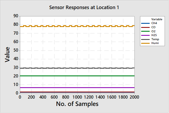Figure 24: Location one sensor responses in field environment testing

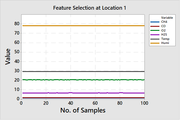Figure 25: Location one feature selection in field environment testing

      Differential baseline manipulation method was used for the air sample data. The baseline data is the different between the reference air and sample data. The process purpose is to remove the outliers and compensate the disturbance effect. This will enhance the data quality and improve sensitivity. Figure 26 shows the instrument baseline manipulation for the location one air sample.

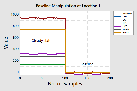Figure 26: Location one baseline manipulation in field environment testing

A normality test was used to investigate the acquired data distribution pattern. The tests used Anderson-Darling (AD), Shapiro-Wilk (SW) and Kolmogorov-Smirnov (KS) methods. The hypothesis for the normality tests was set as:

Null hypothesis, H₀: Data is normal

Alternative hypothesis, H₁: Data is not normal

      The significance level (alpha, α) for AD, SW and KS method was set at 0.05. The results shown in Table 11 indicate that the probability value (p-value) was less than α value for all three normality test methods. As the p-value is less than α, so it will reject the H₀. Thus, the acquired data distribution is not normal and the appropriate method chosen for this data is non-parametric classification analysis.

Table 11: Normality test for AD, SW and KS in field environment testing

	AD	SW	KS
Ambient	<0.005	<0.010	<0.010
Location one	<0.005	<0.010	<0.010
Location two	<0.005	<0.010	<0.010
Location three	<0.005	<0.010	<0.010

      The PCA score plot for field environment testing was shown in Figure 27. Consists of six total PC’s that represent number of instrument sensors and a 2D PCA score plot was used because the first two PC’s variables was 99.42% (PC1 was 97.01% and PC2 was 2.41%) which contain most of the useful information 54. The plot shows that the sample data were clustered into four groups: ambient, location one, location two and location three. The plot indicates the instrument field environment testing’s ability to differentiate air samples at different locations.

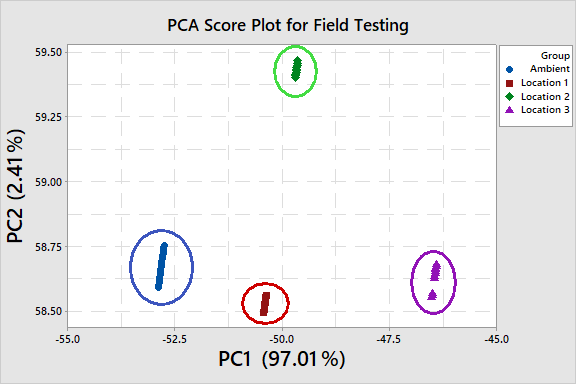Figure 27: PCA score plot for field environment testing

The SVM is a statistical multivariate analysis method that used to test the developed instrument’s capability. The methods robust features are suitable for analysing the sample data. The analysis was conducted to differentiate and classify the samples between ambient (Amb), location one (L1), location two (L2) and location three (L3).

The SVM method used 400 sample data inputs, with 100 acquired from each of the four samples. The train class was set at 70% (280 data) while test class was set at 30% (120 data). The SVM utilised the linear kernel function with prediction speed at 9400 obs/sec, training time at 2.88 sec, automatic kernel scale, box constraint at level one and the multiclass method was one versus one.

      The instrument in field environment test classification success rate is shown by the confusion matrix with 99.28% for train performance and 98.33% for test performance as shown in Table 12. The results indicate that the instrument is successfully being developed and has a high classification success rate in classifying the samples.

Table 12: SVM confusion matrix for e-nose field environment testing

Train Performance						Test Performance
Class		Train Class				Class		Target Class
		Amb	L1	L2	L3			Amb	L1	L2	L3
	Amb	69	1	0	0		Amb	29	1	0	0
	L1	1	69	0	0		L1	1	29	0	0
	L2	0	0	70	0		L2	0	0	30	0
	L3	0	0	0	70		L3	0	0	0	30
Success rate		99.28%				Success rate		98.33%

Table 13: RBFNN confusion matrix for e-nose field environment testing

Train Performance						Test Performance
Class		Train Class				Class		Target Class
		L1	L2	L3	L3			Amb	L1	L2	L3
	Amb	69	1	0	0		Amb	29	1	0	0
	L1	1	69	0	0		L2	1	29	0	0
	L2	0	0	70	0		L3	0	0	30	0
	L3	0	0	0	70		L4	0	0	0	30
Success rate		99.28%				Success rate		98.33%

The RBFNN analysis used 400 sample data inputs, with 100 acquired from each of the four samples. The network used 70% (280 data) of the data for training and the remaining 30% (120 data) for testing. The three-layer feed-forward classification model used six input nodes which corresponds to the instrument sensors includes four MOS sensors, temperature and humidity sensor. The optimum hidden layer neuron also is set to four by using trial and error method. Four neurons were used as the output in sequences of 0001, 0010, 0100 and 1000 to help process the input which implemented the full classifications.

      Table 13 shows the RBFNN classification confusion matrix for the instruments filed environment testing. The instrument classification success rate for classifying four different samples is 99.28% for train performance and 98.33% for test performance. The RBFNN classification result indicates that the instrument is successfully developed and functions accordingly.

7. Conclusion

This work has successfully developed portable e-nose for confined space application. The statistical multivariate analysis and ANN were used to model the air sample in providing potential solutions for the specific confined space application. The major achievement and contributions are summarised.

This work has successfully investigated and identified the atmospheric hazards main hazardous gases (i.e. oxygen, carbon monoxide, hydrogen sulphide and methane) that could contribute to confined space atmospheric accidents. The e-nose sensing module development was based on the main hazardous gases for confined space application.

The e-nose system was successfully fabricated with multimodal sensor detection. The instrument was able to function effectively in providing sample assessment. The instrument’s key features are its portability, ease of operation and effectiveness for use in confined space application.

The e-nose system was successfully integrated with optimum self-purging. The instrument’s self-purging system is able to supply the lowest sensors responses with filtered ambient air for the instrument purging cycle which is important for repeatability.

The e-nose was successfully tested its functionality in the laboratory environment through calibration and validation process using validated instruments includes Altair 5x Multi Gas Detector for concentrations of gases and Humidity Alert meter for temperature and humidity. The 5% percentage error readings between instrument and validated instruments proved its capabilities.

      The e-nose was successfully tested in a real confined space environment (i.e. mechanical room) at Hospital Sultanah Bahiyah (HSB), Alor Setar, Kedah. The instrument is capable of recognizing the concentrations of hazardous gasses at specific locations by discriminated using PCA with a total variation of 99.42%. While the classifiers success rate for SVM and RBFNN indicates of 99.28% for train performance and 98.33% for test performance. The instrument is able to display the atmospheric hazards concentrations in the room which is important during pre-entry testing.

      Finally, based on the achievement of this research work, it is clear that the development of e-nose is able to compete existing devices to accurately and consistently measure atmospheric hazards in confine space applications.

8. Future Work

In order to enhance the instrument capabilities, a number of improvements need to be considered for future work. Firstly, improve the data conversion programming from GUI to embedded system. Secondly, improve the wireless communication distance suitable for a confined space that has a large area. It will ensure a smooth data acquisition process and prevent any data loss.

Thirdly, integrate the acquired data to send into an Internet of Things (IoT) system for real-time remote monitoring.  Finally, integrate the instrument with a mobile robot for ease manoeuvring to various locations in the confined space [56]. This can eliminate an authorised person from entering into the confined space during pre-entry atmospheric testing. The mobile robot should have a complete system with a remote control and charge-coupled device (CCD) camera for any obstacle avoidance.

Acknowledgement

      The author would like to acknowledge the support from the Sciencefund under grant number of 03-01-15-SF0257 from the Ministry of Science, Technology & Innovation Malaysia (MOSTI). The author also gratefully acknowledge to Universiti Malaysia Perlis (UniMAP) for the opportunities given to do the research.

1.  M. A. A. Bakar, A. H. Abdullah, F. S. A. Saad, S. A. A. Shukor, M. S. Kamis, A. A. A. Razak, M. H. Mustafa, “Electronic Nose Purging Technique for Confined Space Application” in IEEE 13th International Colloquium on Signal Processing & its Applications (CSPA), Penang, Malaysia, 2017. DOI: 10.1109/CSPA.2017.8064948.
2.  A. Suruda, T. Pettit, G. Noonan, R. Ronk, “Deadly Rescue: The Confined Space Hazard” Journal of Hazardous Materials, vol. 36, no. 1, pp. 45–53, 1994. https://doi.org/10.1016/0304-3894(93)E0051-3.
3.  Hazards of Confined Spaces. Vancouver: WorkSafeBC, 2008.
4.  H. Ye, “Atmosphere Identifying and Testing in Confined Space” in First International Conference on Instrumentation, Measurement, Computer, Communication and Control, Beijing, China, 2011. DOI: 10.1109.
5.  N. B. A. Wahab, “Fatal Accident Case” Website Department of Occupational Safety and Health Malaysia, Available: http://www.dosh.gov.my/index.php/en/component/content/article/352-osh-info/accident-case/955-accident-case.
6.  T. Suski, “Common Mistakes in Confined Space Monitoring” EHS Today, Available: https://www.ehstoday.com/safety/confinedspaces/ehs_imp_37605.
7.  M. Mamat, S. A. Samad, “The Design and Testing of an Electronic Nose Prototype for Classification Problem” in International Conference on Computer Applications and Industrial Electronics, Kuala Lumpur, Malaysia, 2010. DOI: 10.1109/ICCAIE.2010.5735108.
8.  W. Chansongkram, N. Nimsuk, “Development of a Wireless Electronic Nose Capable of Measuring Odors Both in Open and Closed Systems” Procedia Computer Science, vol. 86, pp. 192–195, 2016. DOI: 10.1016/j.procs.2016.05.060.
9.  F. Röck, N. Barsan, U. Weimar, “Electronic Nose: Current Status and Future Trends” Chemical Reviews, vol. 108, no. 2, pp. 705–725, 2008. DOI: 10.1021/cr068121q.
10.  A. Wilson, M. Baietto, “Applications and Advances in Electronic-Nose Technologies” Sensors, vol. 9, no. 7, pp. 5099–5148, 2009. DOI: 10.3390/s90705099.
11.  RAE Systems by Honeywell, “Application Note 206 Guide to Atmospheric Testing in Confined Spaces” Available: https://www.raesystems.com/sites/default/files/content/resources/Application-Note-206_Guide-To-Atmospheric-Testing-In-Confined-Spaces_04-06.pdf.
12.  L. Capelli, S. Sironi, R. D. Rosso, “Electronic Noses for Environmental Monitoring Applications” Sensors, vol. 14, no. 11, pp. 19979–20007, 2014. DOI: 10.3390/s141119979.
13.  Y. Zou, H. Wan, X. Zhang, D. Ha, P. Wang, Bioinspired Smell and Taste Sensors, Dordrecht: Springer, 2015.
14.  L. Capelli, S. Sironi, R. D. Rosso, “Odor Sampling: Techniques and Strategies for the Estimation of Odor Emission Rates from Different Source Types” Sensors, vol. 13, no. 1, pp. 938–955, 2013. DOI: 10.3390/s130100938.
15.  N. E. Barbri, E. Llobet, N. E. Bari, X. Correig, B. Bouchikhi, “Application of a Portable Electronic Nose System to Assess the Freshness of Moroccan Sardines” Materials Science and Engineering: C, vol. 28, no. 5-6, pp. 666–670, 2008. DOI: 10.1016/j.msec.2007.10.056.
16.  J. Gutiérrez, M. Horrillo, “Advances in Artificial Olfaction: Sensors and Applications,” Talanta, vol. 124, pp. 95–105, 2014. http://dx.doi.org/10.1016/j.talanta.2014.02.016.
17.  T. Pogfay, N. Watthanawisuth, W. Pimpao, A. Wisitsoraat, S. Mogpraneet, T. Lomas, M. Sangworasil, A. Tuantranont, “Development of Wireless Electronic Nose for Environment Quality Classification” in International Conference on Electrical Engineering/Electronics, Computer, Telecommunications and Information Technology (ECTI-CON2010), Chiang Mai, Thailand, 2010.
18.  S. Panigrahi, S. Balasubramanian, H. Gu, C. Logue, M. Marchello, “Design and Development of a Metal Oxide Based Electronic Nose for Spoilage Classification of Beef” Sensors and Actuators B: Chemical, vol. 119, no. 1, pp. 2–14, 2006. DOI:10.1016/j.snb.2005.03.120.
19.  F. Difrancesco, M. Falcitelli, L. Marano, G. Pioggia, “A Radially Symmetric Measurement Chamber for Electronic Noses” Sensors and Actuators B: Chemical, vol. 105, no. 2, pp. 295–303, 2005. DOI:10.1016/j.snb.2004.06.013.
20. A. H. Abdullah, A. H. Adom, A. Y. Shakaff, M. N. Ahmad, M. A. Saad, “Odour Sensor Chamber Development for Electronic Nose” in 4th International Workshop on Computer Science and Engineering-Winter (WCSE), Dubai, UAE, 2014.
21.  S. M. Scott, D. James, Z. Ali, W. T. Ohare, “Optimising of the Sensing Chamber of an Array of a Volatile Detection System: Fluid Dynamic Simulation” Journal of Thermal Analysis and Calorimetry, vol. 76, no. 2, pp. 693–708, 2004. DOI: 10.1023/B:JTAN.0000034891.68585.4a.
22.  D. James, S. M. Scoot, Z. Ali, W. T. O’Hare, “Chemical Sensors for Electronic Nose Systems” Microchima Acta, vol. 149, pp. 1–17, 2005. DOI: 10.1007/s00604-004-0291-6.
23.  G. H. Jain, “MOS Gas Sensors: What Determines Our Choice?” in Fifth International Conference on Sensing Technology (ICST), Palmerston North, New Zealand, 2011. DOI: 10.1109/ICSensT.2011.6137067.
24.  M. Nissfolk, Development of an Electronic Nose-Tongue Data Acquisition System using a Microcontroller, Uppsala University, 2009.
25.  E. Noorsal, O. Sidek, J. M. Saleh, “Automated Odour Measurement in Electronic Nose System Using Microcontroller” in International Conference on Man-Machine Systems 2006, Langkawi, Malaysia, 2006.
26.  A. H. Abdullah, A. H. Adom, A. Y. M. Shakaff, M. N. Ahmad, A. Zakaria, N. A. Fikri, O. Omar, “An Electronic Nose System for Aromatic Rice Classification” Sensor Letters, vol. 9, no. 2, pp. 850–855, 2011. DOI:10.1166/sl.2011.1629.
27.  K.-T. Tang, S.-W. Chiu, M.-F. Chang, C.-C. Hsieh, J.-M. Shyu, “A Low-Power Electronic Nose Signal-Processing Chip for a Portable Artificial Olfaction System” IEEE Transactions on Biomedical Circuits and Systems, vol. 5, no. 4, pp. 380–390, 2011. DOI: 10.1109/TBCAS.2011.2116786.
28.  S. Samadi, “Interface Design Techniques for Electronic Nose Sensors: A Survey” in Sixth International Conference on Advances in Human-oriented and Personalized Mechanisms, Technologies, and Services, Venice, Italy, 2013.
29.  K. M. Pierce, B. Kehimkar, L. C. Marney, J. C. Hoggard, R. E. Synovec, “Review of Chemometric Analysis Techniques for Comprehensive Two Dimensional Separations Data” Journal of Chromatography A, vol. 1255, pp. 3–11, 2012. http://dx.doi.org/10.1016/j.chroma.2012.05.050.
30.  L. A. Berrueta, R. M. Alonso-Salces, K. Héberger, “Supervised Pattern Recognition in Food Analysis” Journal of Chromatography A, vol. 1158, no. 1-2, pp. 196–214, 2007. DOI:10.1016/j.chroma.2007.05.024.
31.  J. Yan, X. Guo, S. Duan, P. Jia, L. Wang, C. Peng, S. Zhang, “Electronic Nose Feature Extraction Methods: A Review” Sensors, vol. 15, no. 11, pp. 27804–27831, 2015. DOI:10.3390/s151127804.
32.  J. Lozano, J. P. Santos, M. C. Horrillo, “Enrichment Sampling Methods for Wine Discrimination with Gas Sensors” Journal of Food Composition and Analysis, vol. 21, no. 8, pp. 716-723, 2008. DOI:10.1016/j.jfca.2008.07.002.
33.  R. Sheebha, M. Subadra, “A Survey on Various Signal Pre-Processing Methods for Sensor Response in E-Nose” Researcher, vol. 6, no. 11, pp. 76–80, 2014. http://www.sciencepub.net/researcher.
34.  N. M. Razali, Y. B. Wah, “Power Comparisons of Shapiro-Wilk, Kolmogorov-Smirnov, Lilliefors and Anderson-Darling tests” Journal of Statistical Modeling and Analytics, vol. 2, no. 1, pp. 21–33, 2011.
35.  N. A. Ahad, T. S. Yin, A. R. Othman, C. R. Yaacob, “Sensitivity of Normality Tests to Non-normal Data” Sains Malaysiana, vol. 40, no. 6, pp. 637–641, 2011.
36.  A. Ghasemi, S. Zahediasl, “Normality Tests for Statistical Analysis: A Guide for Non Statisticians” International Journal of Endocrinology and Metabolism, vol. 10, no. 2, pp. 486–489, 2012. DOI: 10.5812/ijem.3505.
37.  L. I. Smith, A Tutorial on Principal Components Analysis Introduction, 2002.
38.  C. Cortes, V. Vapnik, “Support-Vector Networks” Machine Learning, vol. 20, no. 3, pp. 273-297, Kluwer Academic Publishers, 1995.
39.  Z. Haddi, A. Amari, H. Alami, N. El Bari, E. Llobet, B. Bouchikhi, “A Portable Electronic Nose System for the Identification of Cannabis-based Drugs” Sensors and Actuators B: Chemical, vol. 155, no. 2, pp. 456-463, 2011. DOI: 10.1016/j.snb.2010.12.047.
40.  L. Auria, R. A. Moro, “Support Vector Machines (SVM) as a Technique for Solvency Analysis” SSRN Electronic Journal, 2008. DOI: 10.2139/ssrn.1424949.
41.  I.-C. Chen, J. K. Hill, R. Ohlemuller, D. B. Roy, C. D. Thomas, “Rapid Range Shifts of Species Associated with High Levels of Climate Warming” Science, vol. 333, no. 6045, pp. 1024–1026, 2011. DOI: http://ssrn.com/abstract=1424949.
42.  R. Domínguez, L. Moreno-Barón, R. Muñoz, J. Gutiérrez, “Voltammetric Electronic Tongue and Support Vector Machines for Identification of Selected Features in Mexican Coffee” Sensors, vol. 14, no. 9, pp. 17770–17785, 2014. DOI: 10.3390/s140917770.
43.  J. Brezmes, N. Canyellas, E. Llobet, X. Vilanova, X. Correig, “Application of Artificial Neural Networks to the Design and Implementation of Electronic Olfactory Systems” in 5th Seminar on Neural Network Applications in Electrical Engineering (NEUREL 2000), Belgrade, Yugoslavia, 2000. DOI: 10.1088/0957-0233/1/5/012.
44.  T. Li, “The Application of Artificial Neural Networks in the Electronic Nose for Odour Measurement,” M.Sc. Thesis, University of Manitoba, 2005.
45.  K. Suzuki, Artificial Neural Networks – Industrial and Control Engineering Applications, Rijeka: InTech, 2011.
46.  C. S. Kudarihal, M. Gupta, “Electronic Nose Based on Metal Oxide Semiconductor Sensors as an Alternative Technique for Perception of Odours” International Journal of Advances in Engineering & Technology, vol. 7, no. 1, pp. 206–216, 2014.
47.  M. Ghasemi-Varnamkhasti, S. S. Mohtasebi, M. Siadat, S. Balasubramanian, “Meat Quality Assessment by Electronic Nose (Machine Olfaction Technology)” Sensors, vol. 9, no. 8, pp. 6058–6083, 2009. DOI: 10.3390/s90806058.
48.  B. Tudu, A. Jana, A. Metla, D. Ghosh, N. Bhattacharyya, R. Bandyopadhyay, “Electronic Nose for Black Tea Quality Evaluation by an Incremental RBF Network” Sensors and Actuators B: Chemical, vol. 138, no. 1, pp. 90–95, 2009. DOI: 10.1016/j.snb.2009.02.025.
49.  H. D. Leon-Delgado, R. J. Praga-Alejo, D. S. Gonzalez-Gonzalez, M. Cantú-Sifuentes, “Multivariate Statistical Inference in a Radial Basis Function Neural Network” Expert Systems with Applications, vol. 93, pp. 313–321, 2018. DOI: 10.1016/j.eswa.2017.10.024.
50.  N. P. Thanh, Y.-S. Kung, S.-C. Chen, H.-H. Chou, “Digital Hardware Implementation of a Radial Basis Function Neural Network” Computers & Electrical Engineering, vol. 53, pp. 106–121, 2016. http://dx.doi.org/10.1016/j.compeleceng.2015.11.017.
51.  K. Wetchakun, T. Samerjai, N. Tamaekong, C. Liewhiran, C. Siriwong, V. Kruefu, A. Wisitsoraat, A. Tuantranont, S. Phanichphant, “Semiconducting Metal Oxides as Sensors for Environmentally Hazardous Gases” Sensors and Actuators B: Chemical, vol. 160, no. 1, pp. 580–591, 2011. DOI: 10.1016/j.snb.2011.08.032.
52.  M. A. A. Bakar, A. H. Abdullah, F. S. A. Sa’Ad, S. A. A. Shukor, M. H. Mustafa, M. S. Kamis, A. A. A. Razak, S. A. Saad, “Electronic Nose Sensing Chamber Design for Confined Space Atmospheric Monitoring” in International Conference on Mathematics, Engineering and Industrial Applications 2016 (ICoMEIA), Songkhla, Thailand, 2016. http://dx.doi.org/10.1063/1.4965179.
53.  M.A.A. Bakar, A.H. Abdullah, F.S.A. Sa’ad, S.A.A. Shukor, A.A.A. Razak, M.H. Mustafa, “Electronic Nose Calibration Process for Monitoring Atmospheric Hazards in Confined Space Applications” Journal of Telecommunication, Electronic and Computer Engineering (JTEC), 2016.
54.  A. F. Najmuddin, I. M. Ibrahim, S. R. Ismail, “A Simulation Approach: Improving Patient Waiting Time for Multiphase Patient Flow of Obstetrics and Gynecology Department (O&G Department) in Local Specialist Centre” WSEAS TRANSACTIONS on MATHEMATICS, vol. 9, no. 10, pp. 778–790, 2010.
55.  K.-T. Tang, S.-W. Chiu, C.-H. Pan, H.-Y. Hsieh, Y.-S. Liang, S.-C. Liu, “Development of a Portable Electronic Nose System for the Detection and Classification of Fruity Odors” Sensors, vol. 10, no. 10, pp. 9179–9193, 2010. DOI: 10.3390/s101009179.
56.  H. Ishida, Y. Wada, H. Matsukura, “Chemical Sensing in Robotic Applications: A Review” IEEE Sensors Journal, vol. 12, no. 11, pp. 3163–3173, 2012. DOI: 10.1109/JSEN.2012.2208740.

(Click Here)

(Click Here)