1. Introduction

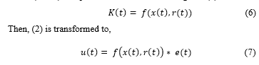
There have been growing demands for autonomous vehicles with excellent maneuvering capabilities both for commercial and military applications [1, 2]. Significant amount of work is ongoing to realize the commercial operation of autonomous cars [3, 4], and Wheeled Mobile Robots (WMRs) are finding increasing use in industrial and service applications [5]. Autonomous Surface Vehicles (ASV) have been utilized to improve port safety and for ecological as well as meteorological purposes [6], whereas Autonomous Underwater Vehicles (AUVs) are useful tools for underwater search and inspection [7].

Safe navigation will require both excellent path planning and path tracking strategies. Path planning involves the determination of an appropriate trajectory for the vehicle whereas path tracking, which is the focus of this study, is the following of a desired trajectory. Several schemes have been reported in the literature for path planning, including in [8], where a framework was proposed to synthesize sequences of maneuvers that are tracked using nonlinear controllers, and other strategies are presented in [9, 10]. To execute the maneuvers generated by path planners, control strategies have been proposed as well.

In [11], Fuzzy Logic Controller (FLC) was proposed for robot tracking and Proportional-Integral-Derivative (PID) controller was utilized to control the speed of WMRs in [12]. The authors of [13] presented an observer-based approach, whereas backstepping control strategy was presented in [14, 15]. Sliding-mode control for WMR trajectory tracking with initial error was reported in [16], and modular-based method was proposed in [17]. The authors of [18] proposed a Model Predictive Control (MPC) approach and Kalman filter-based strategy was presented in [19]. Lyapunov-based scheme was reported in [20] and controller design by approximate linearization utilizing Taylor expansion was proposed in [21]. In order to enhance the perfomance of traditional control methods, Least Square Policy Iteration (LSPI) and Dynamic Heuristic Programming (DHP) algorithms were utilized in [22] for optimizing a Proportional-Derivative (PD) controller. Also, the authors of [23] utilized neural network (NN) to describe the inverse dynamics of a biped robot with respect to output errors for the control of level walking. However, application examples were limited to scenarios where the robot is initialized at the desired starting coordinate.

In order to execute maneuvers for unmanned Air Vehicles (UAVs), feedback linearization [24, 25] and sliding mode control [26] have been proposed, but they have failed for certain models due to the nonlinear dynamics of the vehicle [27]. For helicopter control, backstepping control strategy [28] and Linear Quadratic Regulator (LQR)-based control [29] have been proposed.

In this study, a novel learning-based adaptive scheme utilizing the neural network is developed for autonomous vehicle trajectory tracking. Whereas, plant models predict the vehicular motion for a given control command, accuracy is limited by modelling errors and approximations. Also, for certain models with complex nonlinear dynamics, it is difficult to obtain a suitable controller. Since machine learning models provide a more powerful tool to describe nonlinear dynamics of a plant given example data of plant operation, this article presents a parameterized control law designed to achieve trajectory tracking of autonomous vehicles adaptively. Rather than using a single controller, a family of controllers is obtained utilizing the NN model to estimate the time varying controller parameters. The scheme was applied to optimize a Lyapunov-based nonlinear controller parameters used to execute an eight-shaped maneuver for a mobile robot. Furthermore, LQR-based controller parameters for 2-Degree-Of-Freedom (DOF) helicopter position control were optimized using the proposed scheme. Simulation results show that the scheme outperforms the traditional control strategies in terms of faster convergence to the desired trajectory and more accurate steady-state performance, regardless of the initial shift in starting coordinates. Also, because the scheme is sample-based, it can compensate for modeling errors.

The rest of the paper is organized as follows; Section 2 presents the problem formulation. Section 3 provides an illustrative application of the proposed scheme. Simulation results are discussed in Section 4, and Section 5 summarizes the study.

2. Problem Formulation

A dynamic system can generally be defined in state-space as,

The system state is represented by , the control input is denoted by , whereas  denotes a mathematical function and    is the state derivative with respect to time. Given a target signal , a traditional feedback control law can be computed based on the difference between the target signal and the actual system output. Such difference can be denoted by , resulting in a control input defined as,

where  denote the control gain, which can be constant or time-varying depending on the dynamic description of the system. However, by utilizing certain control strategies, not only the error is fed back for control but the states also. For two-dimensional and higher order systems; the states, control input and error signals are vectors, whereas the control gain could be a vector or matrix depending on the control strategy used.

      In order to optimize the controller performance for changing system dynamics or operation regions, a neural network-based method that adaptively determines the control gain is proposed as follows. For a traditional closed-loop control system, sample test run of the system is performed and for each time step , the state variables and the control gain are measured and arranged into 3-tuple The state measurement before the application of control input is denoted as  whereas the next state caused by the control action is. The control gain that caused the state transition is represented as

      Multiple samples of state transitions and control gains are measured for a sequence of operation, then the control gain or the control gain parameters for time-invariant or time-varying system respectively are varied for other sequences. Example of a sequence is the tracking of a particular course by a mobile robot or the change in angular orientation of a helicopter over a period of time. For training stability, the data set is normalized depending on the data range. And based on the accumulated data set as represented by the 3-tuple, a NN is trained using the state and next state as input and the control gain as the output. Hence,

      The NN model is made up of processing units called neurons with weighted interconnections among them [30], and the neurons with nonlinear activation functions are arranged into layers as shown in Figure 1.

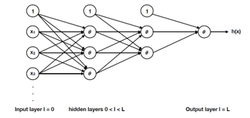Figure 1: Feed forward neural network structure

The input layer is the vector of input variables, which are system states in the study. For a single hidden layer system, the hidden layer is a nonlinear combination of the input signals, and for multiple hidden layer system, subsequent layers are nonlinear combination of the previous layers. Knowledge is extracted from the output layer after model training. In supervised learning employed in this study, an error function based on the difference between the actual outputs called labels and the predicted outputs from the NN is minimized to adjust the interconnection weights among the neurons. After several iterations, the model is said to be trained. Whereas only a portion of the dataset is used for training, the remainder is used for testing the performance of the trained model. The mathematical description of the NN model as utilized in this study is,

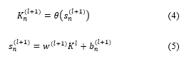
      where the output vector of a layer is denoted by . Hence, the input layer vector  is equivalent to the state input  The activation function is denoted by  and  represents the input vector to layer . The interconnecting weights and biases from layer  to unit  of layer   are represented by  and  respectively.

      Following offline training as decribed above, the trained NN model is integrated as a control gain estimator in the traditional control system as shown in Figure 2.

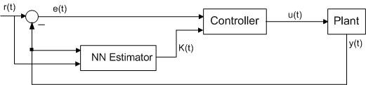Figure 2: Neural network optimized adaptive control system

For online control gain estimation, the NN input due to the next state  is replaced with the reference signal . Hence,

3. Illustrative Examples

      In order to prove the effectiveness of the proposed scheme, two application case studies are presented. One is the tracking of an eight-shaped trajectory by a mobile robot, and the other is the position tracking of a 2-DOF helicopter.

3.1.  Mobile Robot Trajectory Tracking

      The nonlinear kinetic model [31] of a non-holonomic wheeled mobile robot is described as,

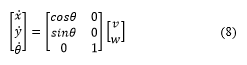      The robot’s states    are the cartesian and angular displacements respectively. Whereas  and are the state derivatives,  corresponds to the linear velocity and  represents the angular velocity around the vertical axis.

3.1.1. Traditional Control Design

      Motion control of the mobile robot is achieved by computing appropriate linear and angular velocities to drive the robot in the desired trajectory. According to the procedure in [32], the state tracking error is generalized by defining it through a rotation matrix to obtain,

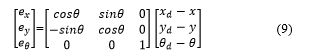where ,   and  are the target coordinates for the robot. Then the error dynamics in generalized coordinates is obtained by taking the derivative of (9) as,

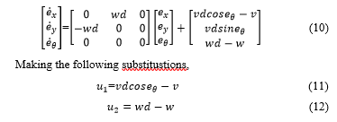The error dynamics is transformed to the subsequent form,

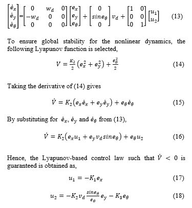
The controller gains are defined as,

where  is 0 or 1 for forward or backward motion respectively. The feedback commands are adaptively computed based on NN estimation as described next.

3.1.2. Controller Parameter Estimation using the Neural Network

      In order to optimize the controller for fast convergence to the desired trajectory and improved steady-state performance, the NN is utilized to adaptively estimate the feedback control parameters. Sample runs of the traditional closed-loop system are performed for 15 sequences of 1258 state transitions to make a total of 18870 data samples. The input features are the current state , the nominal velocities [ and the next state   The output labels are the control gains [     ] responsible for the state transition. Data was normalized and the training was implemented using the MATLAB NN tool box using 70% of the dataset. The remaining dataset was divided into 15% validation and 15% testing. The Levenberg-Marquerdt algorithm [33, 34, 35] was used for training using two hidden neurons. The performance of the NN estimator was evaluated using the Mean Square Error (MSE) plot shown in Figure 3. The figure shows good generalization performance as the test error is approximately equal to that of the training.

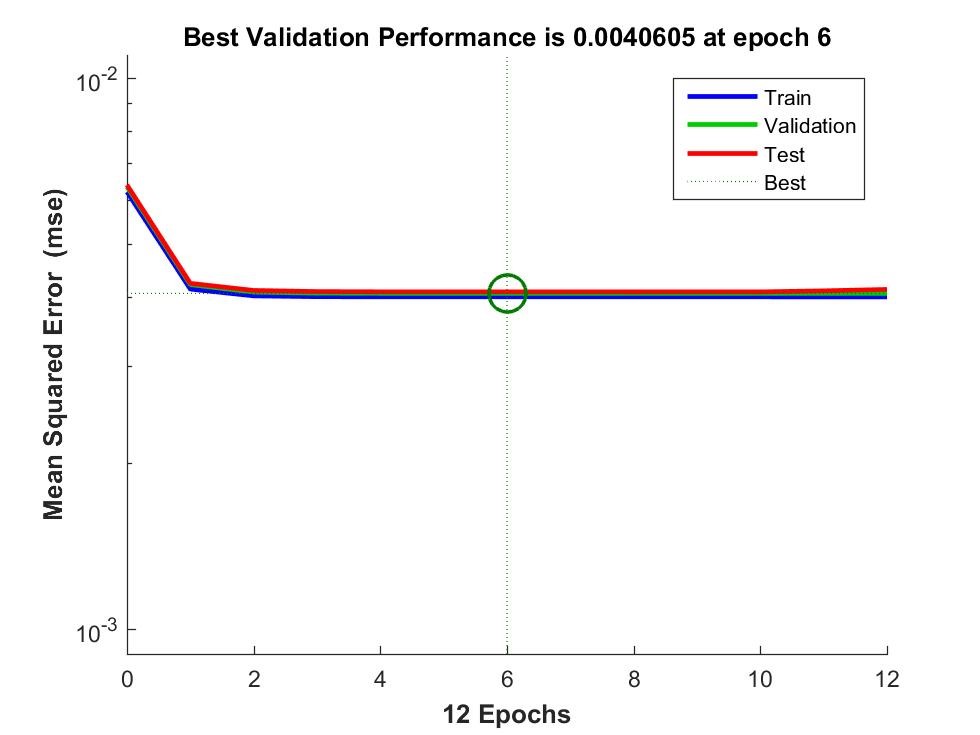Figure 3: MSE of the NN estimator for robot control

      The trained NN estimator is integrated in the second loop of Figure 2, where a normalizer and denormalizer are embedded for better control performance. Simulation results of the adaptive closed loop control system is presented in Section 4.

3.2.    2-DOF Helicopter Position Control

A Two-Input-Two-Output (TITO) Quanser 2D Helicopter model [35] is considered. The linearized model is obtained in [36] as follows.

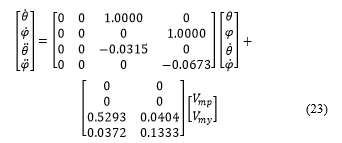where  and  are the pitch and yaw angles respectively.The first and second derivatives of the pitch and yaw angles are respetively. The pitch and yaw propeller voltages  and  are applied to the corresponding motors driving the propellers.

3.2.1. Traditional Control Design

The pitch and yaw angles of the 2-DOF helicopter were regulated using the optimal LQR-based control design presented in [29]. And the control law was obtained as,

The realized state feedback gains are,

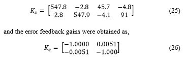
 The system states are represented by  whereas  is the error feedback signal. The adaptive computation of the error feedback gains using the NN is subsequently described.

3.2.2. Controller Parameter Estimation using the Neural Network

      In order to achieve better accuracy and faster tracking convergence, the NN is employed to optimize the error feedback control gains. In this case, six sequences of 700 state transitions totaling 4195 data samples were sufficient, since the plant has been linearized. The input features are the current angular orientation along with the next angular orientation  of the 2-DOF helicopter. The output labels are the error feedback control gains responsible for the angular orientation change. Similar procedures as proposed in Subsession 3.1.2 of this paper are followed, and the MSE plot is as shown in Figure 4. The figure shows good generalization of the estimator similar to observation in the previous section since the test error approximates the training error. The trained NN estimator is integrated in the second loop of Figure 2 to obtain optimized performance as presented next in Section 4.

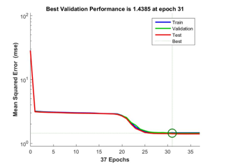Figure 4: MSE of the NN estimator for helicopter control

4. Simulation Results

Closed-loop simulation was conducted in Matlab Simulink for both the traditional and the NN-optimized control system. The results for different initial state shifts were compared to prove the effectiveness of the proposed scheme. The desired eight-shaped trajectory for the mobile robot was defined as,

The feed-forward driving and steering velocities as described by (20) and (21) are shown in Figures 5 and 6 respectively.

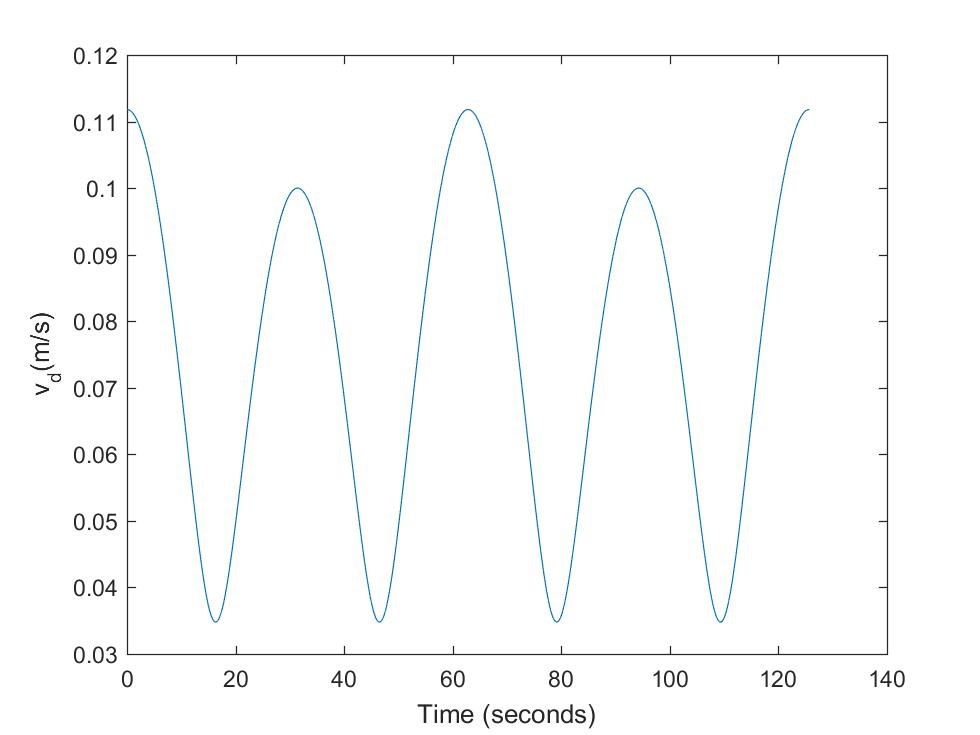Figure 5: Robot feed-forward driving velocity input

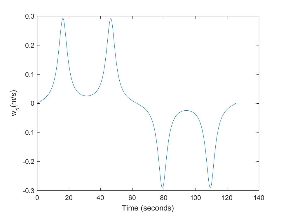Figure 6: Robot feed-forward steering velocity input

Figures 7 – 9 is the trajectory tracking performance of the nonlinear Lyapunov-based controller for the mobile robot with initial state error , where the linear displacement unit is meters and radians is the unit of the angular displacement. Figure 7 is the result of an underdamped control system due to low damping ratio, whereas Figure 8 is the result of an over-damped control system due to high damping ratio. The result of a critically damped control system with unity damping ratio is shown in Figure 9, whereas Figure 10 is the corresponding trajectory tracking output performance of the NN-optimized control system. It can be observed that the NN-optimized controller outperformed the different design modes of Lyapunov-based controller in terms of faster convergence to the desired trajectory and steady-state error minimization. The steady-state is the region starting at the point where the robot settles around the reference trajectory.  Although, either fairly good convergence or steady-state performance can be obtained by varying the control parameters of the Lyapunov-based controller, but the improvement is mutually exclusive. However, the NN-optimized controller achieved both better transient and steady state performances concurrently by adaptively obtaining varying controller parameters.

Figures 11 – 14 are the control performance outputs for the mobile robot trajectory tracking with initial state error . Also in this case, linear and angular displacements are measured in meters and radians respectively. It can be observed, as the case is in the previous example, that the NN-optimized controller of Figure 14 showed better comparative control performance than the different variations of traditional Lyapunov-based controllers of Figures 11 – 13.

To further show the performance advantage of the NN-optimized controller, the average linear and angular tracking errors over the entire trajectory are presented in Table 1 as it applies to the different initial state errors. It can be seen that both the resultant linear and angular tracking errors are minimized using the NN-optimized controller.

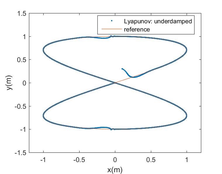Figure 7: Underdamped robot Lyapunov-based control

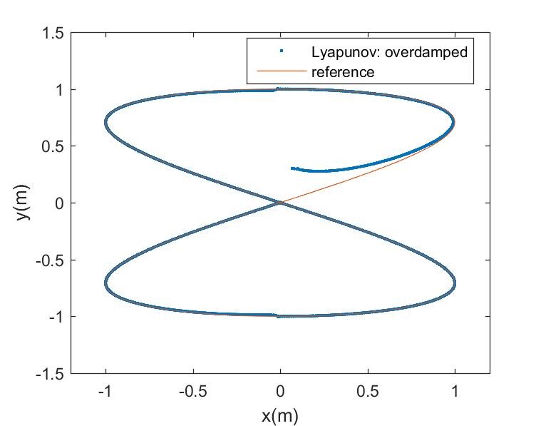Figure 8: Overdamped robot Lyapunov-based control

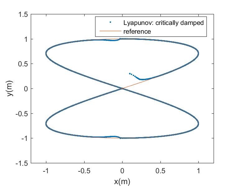Figure 9: Critically damped robot Lyapunov-based control

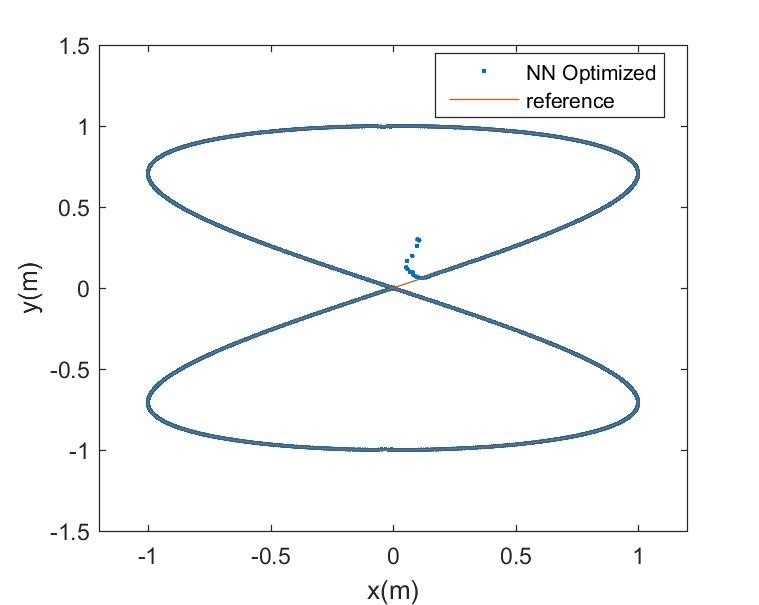Figure 10: Robot NN-optimized control

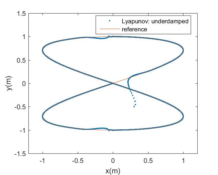Figure 11: Underdamped robot Lyapunov-based control

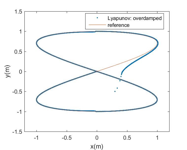Figure 12: Overdamped robot Lyapunov-based control

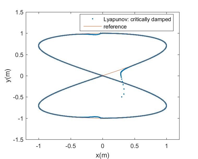Figure 13: Critically damped robot Lyapunov-based control

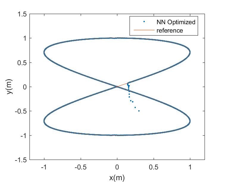Figure 14: Robot NN-optimized control

Table 1: Robot mean tracking error based on control method

Control Method	Initial state error [m,m,rad]	Mean x error (m)	Mean y error (m)	Mean θ error (m)
Lyapunov_ underdamped	[0.1,0.3,0]	1.7×10-3	-2.3×10-3	2.4×10-2
Lyapunov_ overdamped	[0.1,0.3,0]	-1.8×10-4	-9.2×10-3	2.3×10-2
Lyapunov_ critically damped	[0.1,0.3,0]	2.8×10-4	-3.8×10-3	2.6×10-2
Neural network optimized	[0.1,0.3,0]	3.5×10-4	-2.5×10-4	2.2×10-2
Lyapunov_ underdamped	[0.3,-0.5,π/6]	3.5×10-3	2.1×10-3	-2.1×10-2
Lyapunov_ overdamped	[0.3,-0.5,π/6]	4.4×10-4	1.33×10-2	-3.5×10-2
Lyapunov_ critically damped	[0.3,-0.5,π/6]	1.4×10-3	4.1×10-3	-2.3×10-2
Neural network optimized	[0.3,-0.5,π/6]	-5.1×10-4	-1.3×10-4	-3.3×10-2

The desired positioning of the 2-DOF helicopter pitch and yaw angular orientations over time are defined as,

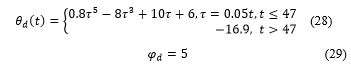
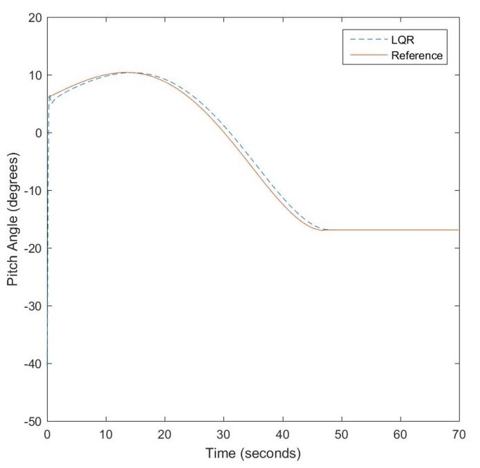Figure 15: LQR-based pitch angle control

The LQR-based controller performance is shown in Figures 15 and 17 with initial pitch and yaw angular orientations of -40.5 and 0 degrees. The Q and R parameters were selected as  and  where Q is associated with both the state and error feedback signals. The performances of the NN-optimized controller are shown in Figures 16 and 18 for pitch and yaw angle control respectively. Since the system is linearized, modest performance improvement is observed with respect to response speed and steady-state error minimization. Table 2 shows the comparative tracking errors.

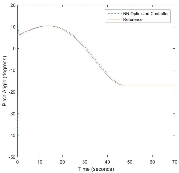Figure 16: NN-optimized pitch angle control

Figure 17: LQR-based yaw angle control

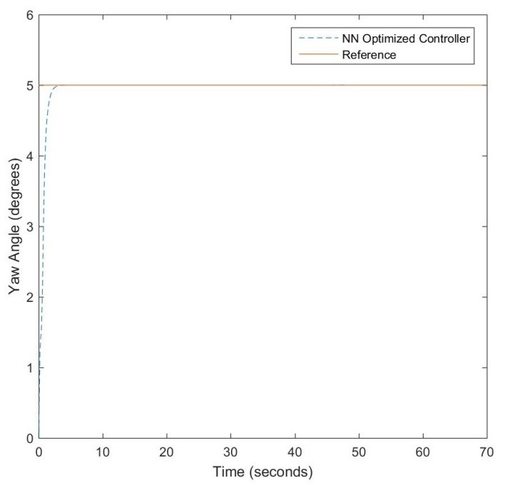Figure 18: NN-optimized yaw angle control

Table 2: Helicopter mean tracking error based on control method

Control Method	Initial state error (degrees)	Mean θ error (degrees)	Mean φ error (degrees)
LQR	[-40.5,0]	-0.18	0.08
Neural network optimized	[-40.5,0]	-0.06	0.04

5. Conclusion

A neural network optimized control system design for autonomous vehicle navigation has been proposed in this study. The design consists of an inner error loop integrated with an outer loop for estimating the controller parameters utilizing a neural network trained on samples from test navigation. Comparative studies of the proposed scheme with traditional methods were presented. In the first case, the neural network optimized control system was shown to outperform a Lyapunov-based controller in terms of faster convergence to the desired trajectory and better steady-state performance for an eight-shaped maneuver. A second illustrative simulation example was conducted for the control of pitch and yaw angles of a 2-Degree-Of-Freedom helicopter model, where improved transient and steady-state performances were observed for NN-optimized controller over a Linear Quadratic Regulator-based controller.

Because the neural network structure allows complex and nonlinear mapping of variables, the trained estimator is able to learn the behavior of both linear and nonlinear systems. Furthermore, since the proposed scheme is sample-based, it can compensate for plant modelling errors that degrades the performance of traditional controllers in real-life applications.

Conflict of Interest

The authors declare no conflict of interest.

Acknowledgment

The research work presented in this article is supported in part by the US National Science Foundation award 1464387, 1736196 and by the U.S. Office of the Under Secretary of Defense for Research and Engineering (OUSD(R&E)) under agreement number FA8750-15-2-0119. The U.S. Government is authorized to reproduce and distribute reprints for governmental purposes notwithstanding any copyright notation thereon. The views and conclusions contained herein are those of the authors and should not be interpreted as necessarily representing the official policies or endorsements, either expressed or implied, of the US National Science Foundation or the Office of the Under Secretary of Defense for Research and Engineering (OUSD(R&E)) or the U.S. Government.

1.  S. Thrun, M. Montemerlo, H. DahlKamp, D. Stavens, A. Aron, J. Diebel, P. Fong, J. Gale, M. Halpenny, G. Hoffman et al, “Stanley: The robot that won the DARPA grand challenge”. J. Field Robot, 23(9), 661-692, 2006
2.  D. Weatherington, Unmanned Aerial Vehicle Roadmap Report, The Information Warfare Site, 2003. http://www.iwar.org.uk/news-archive/2003/03-18-5.htm
3.  T. Luettel, M. Himmelsbach, H. J. Wuensche, “Autonomous ground vehicles-concepts and a path to the future” in Proc. of the IEE, 100 (Special Cantennial Issue), 1831-1839, 2012. https://doi.org/10.1109/JPROC.2012.2189803
4.  T. Drage, J. Kalinowski, T. Braunl, “Integration of drive-by-wire with navigation control for a driverless electric race car” IEEE Intelligent Transportation Systems Magazine, 6(4), 23-33, 2014. https://doi.org/10.1109/MITS.2014.2327160
5.  R. D. Schratt, G. Schmierer, Serviceroboter, Springer, Berlin, 1998
6.  N. Miskovic, D. Nad, L. Rendulic, “Tracking divers: An autonomous marine surface vehicle to increase diverse safety” IEEE Robotics Automation Magazine, 22(3), 72-84, 2015. https://doi.org/10.1109/MRA.2015.2448851
7.  F. Plumet, C. Petres, M.A. Romero-Ramirez, B. Gas, S.H Long, “Toward and autonomous sailing boat” IEEE Journal of Oceanic Engineering, 40(2), 397-407, 2015. https://doi.org/10.1109/JOE.2014.2321714
8.  E. Frazzoli, M.A. Dahleh, E. Feron, “Maneuver based motion planning for nonlinear systems with symmetries” IEEE Trans. Robot. Automat., 21, 1077-1091, 2005. https://doi.org/10.1109/TRO.2005.852260
9.  C. Dever, B. Mettler, E. Feron, J. Popovic, M. McConley, “Nonlinear trajectory generation for autonomous vehicles via parameterized maneuver classes” J. Guid. Control Dyn., 29(2), 289-302, 2006 https://doi.org/10.2514.1.13400
10.  N. K. Ure, G. Inalhan, “Autonomous Control of unmanned combat air vehicles: design of a multimodel control and flight planning framework for agile maneuvering” IEEE Control Systems Magazine, 32(5), 74-95, 2012. https://doi.org/10.1109/MCS.2012.2205532
11.  S. Qiu, Z. Li, W. He, L. Zhang, C. Yang, C. Y. Su, “Brain-machine interface and visual compressive sensing-based teleoperation control of an exoskeleton robot” IEEE Trans. On Fuzzy Systems, 25(1), 58-69, 2017. https://doi.org/10.1109/TFUZZ.2016.2566676
12.  C. S. Shijin, K. Udayakamar, “Speed control of wheeled mobile robots using pid with dynamics and kinetic modelling” in 4th International Conference on Innovations in Information, Embedded and Communication Systems (ICIIECS), 1-7, 2017. https://doi.org/10.1109/ICIIECS.2017.8275962
13.  M. Chen, “Disturbance attenuation tracking control for wheeled mobile robots with skidding and slipping” IEEE Trans. On Industrial Electronics, 64(4), 3359-3368, 2017. https://doi.org/10.1109/TLE.2016.2613839
14.  W. M. E. Mahgoub, I. M. H. Sanhoury, “Back stepping tracking controller for wheeled mobile robot” in Proc. of International Conference on Communications, Control, Computing and Electronics Engineering (ICCCCEE), 1-5, 2017. https://doi.org/10.1109/ICCCCEE.2017.7867663
15.  O. Chwa, “Slidding-mode tracking control of nonholonomic wheeled mobile robots in planar corrdinates” IEEE Trans. Control Syst. Technol., 12, 637-666, 2004. https://doi.org/10.1109/TCST.2004.824953
16.  Z. Jiang, H. Nijmeijer, “Tracking control of mobile robots: a case study in backstepping” Automatica, 33, 1393-1399, 1997 https://doi.org/10.1016/50005-1098(97)00055-1
17.  M. M. Michalek, “Cascade-like modular tracking controller for non-standard N-Trailers” IEEE Trans. On Control Systems Technology 25(2), 619-627, 2017 . https://doi.org/10.1109/TCST.2016.2557232
18.  H. Yang, M. Guo, Y. Xia, L. Cheng, “Trajectory tracking for wheeled mobile robots via model predictive control with softening constraints”. IET Control Theory and Applications, 12(2), 206-214, 2018. https://doi.org/10.1049/iet.cta.2017.0395
19.  M. Cui, W. Liu, H. Liu, X. Lu, “Unscented Kalman filter-based adaptive tracking control for wheeled mobile robots in the presence of wheel slipping” in Proc. 12th World Congress on Intelligent Control and Automation (WCICA), 3335-3340. https://doi.org/10.1109/WCICA.2016.7578636
20.  Y. Wang, Z. Miao, H. Zhong, Q. Pan, “Simultaenous stabilization and tracking of nonholonomic mobile robots: a lyapunov-based approach” IEEE Trans. On Control Systems Techonology, 23(4), 1440-1450, 2015 https://doi.org/10.1109/TCST.2014.2375812
21.  F. Kuhne, W. F. Lages, J. M. G. da Silva, L. Jono “Model predictive control of a mobile robot using linearization” in Proc. Mechatronics and Robotics, 2004.
22.  H. Yang, Q. Guo, X. Xu, C. Lian, “Self-learning pd algorithms based on approximate dynamic programming for robot motion planning” in 2014 International Joint Conference on Neural Networks (IJCNN), 3663-3670, 2014. https://doi.org/10.1109/IJCNN.2014.6889711
23.  J. K. Rai, V. P. Singh, R. P. Tawari, D. Chandra, “Artificial Neural Network controllers for biped robot” 2nd International Conference on Power, Control and Embedded Systems, 625-630, 2012. https://doi.org/10.1109/ICPCES.2012.6508093
24.  A. Isidori, Nonlinear Control Systems, M. Thoma, Ed., Springer NewYork, 1995.
25.  S. Sastry, Nonlinear Systems, J. E. Marsden, L. Sirovich, S. Wiggins, Eds., Springer New York, 1999.
26.  V. I. Utkin, Sliding Modes in Control and Optimization, Springer Berlin, 1992
27.  J. J. E Slobine, W. Li, Applied Nonlinear Control, Prentice Hall, Englewood Cliffs, NJ, 1991
28.  E. Frazzoli, M. Dahleh, E. Feron, “Trajectory tracking control design for autonomous helicopters using backstepping algorithm” in Proc. American Control Cont., 6, 4102-4107, 2000. https://doi.org/10.1109/ACC.2000.876993
29.  X. Meng, Y. Zhang, J. Zhang, “Multiple input/ouput delays compensation for networked mimo systems” in 25th Chinese Control and Decision Conference (CCDC), 2545-2550, 2013. https://doi.org/10.1109/CCDC.2013.6561369
30.  Y. S. Abu-Mostafa, M. Magdon-Ismail, H. Lin, Learning from Data, AMC book.com, USA, 2012.
31.  S. Blazic, “Two approaches for nonlinear control of wheeled mobile robots” in 13th IEEE International Conference on Control Automation (ICCA), 946-951, 2017. https://doi.org/10.1109/ICCA.8003188
32.  A. D. Luca, G. Oriolo, M. Venditteli, Control of Wheeled Mobile Robots: An Experimental Overview In: S. Nicosia, B. Siciliano, A. Bicchi, P. Valigi (eds) Ramsete. Lecture Notes in Control and Information Sciences, 270, Springer, Berlin, Heidelberg, 2001.
33.  K. Levenberg, “A method for the solution of certain problems in least square” Quart. Appl. Math., 2, 164-168, 1944. https://doi.org/10.1109 /qam/10666
34.  D. Marquerdt, “An algorithm for least-square estimation of linear parameters” SIAM J. Appl. Math., 11(2), 431-441, 1963. https://dx.doi.org/10.1137/0111030
35.  A. Ranganathan, “The Levenberg-Marquardt Algorithm”. Honda Research Institute USA, 2004. http://ananth.in/Notes-files/Imtut.pdf
36.  Quanser 2 DOF Helicopter User and Control Manual. Quanser Inc., Canada, 2006.

(Click Here)

(Click Here)