1. Introduction

This paper is an extension of the article presented at the IEEE International Symposium on Signal Processing and Information Technology [1]. Here and there we address the task of robotic catching of thrown objects or, more precisely the subtask of observing and predicting the trajectory of the thrown object.

With the development of robotics, mechanical systems acquire more and more features that were previously only available to humans. One of these possibilities is the ability to catch objects thrown in the air. Initially, a robotic capture of objects thrown in the air was described in 1991 in [2]. Later, this task was considered several times in a number of articles [1,3,11].

In addition to theoretical value, such a skill can have a practical application. For example, in light industry, the task of transporting workpieces between machine tools processing them often arises. The traditional solution to this problem is the use of various conveyor systems. Robotic transfer as a method of such transportation was proposed in 2006 by Frank [12]. This application was developed in [13-21]. Transportation of an object from some point of departure A to some destination B is as follows: the robot thrower located in A throws the object in direction B and notifies about it via the communication line, and the robot catcher located in B, having received the notification, carries out object capture on the fly.

The authors of [12,15] specify the following potential advantages of robotic throw compared to traditional conveyor-based systems:

• Greater flexibility. Flexibility is understood as the ability to quickly deploy, collapse and redevelop a transport network with an arbitrary topology, or to use it in production facilities with an arbitrary layout.
• Higher speed of object transportation.
• Reduced energy consumption.

The share of successful captures in most existing systems does not exceed 80% (two exceptions are described in [11] and [16]; in the first article, a high proportion of successful captures is provided by large linear dimensions of the gripping device; in the second, by throwing cylindrical objects of high aerodynamic stability), which is not sufficient for use in a real industrial environment. Thus, the practical implementation of transportation by robotic throw is a complex and relevant scientific task.

For a successful capture, it is necessary to know in which point of space the object will be at the moment of capture, and at what speed it will move at the same time [15]. The point in space and time where the capture is carried out is selected among the set of points that the object passes when it flies through the working space of the capture device. Their combination forms the trajectory of the object in the working space of the capture device. This trajectory must be predicted in advance so that the robot catcher has time to complete the capture [15]. Prediction is based on measuring the object trajectory immediately after the throw. In general, in [15], the following four subtasks are distinguished when ensuring the transportation of objects by robotic transfer:

• throw;
• capture;
• forecasting;

Here we consider last two subtasks. Trajectory forecasting is needed in order to provide the catcher with the information about object trajectory within the workspace of the gripper. Most of the trajectory forecasting algorithms are based on ballistic modeling of the flight. These models include the influence of gravitation only (e. g. [2,3,7]; in this case forecasting may be implemented by fitting a parabola to the reference of measured positions) or gravitation and air drag (e. g. [4,8,9]). This modeling requires preliminary knowledge about ballistic properties of thrown objects. However, human children do not need such a knowledge to catch the ball successfully. They do it only based on the previous experience. This circumstance motivated the development of learning-based forecasting algorithms, such as neural network trajectory predictor [18] and k nearest neighbor’s trajectory predictor [19-21]. Learning-based techniques require collecting the sampling of trajectories in order to train the predictor. Here we propose the method, which lies between model-based and learning-based model. The predictor is using equations to define future positions of the object, but the parameters of these equations are obtained by the learning procedure of genetic programming. Learning does not require a sampling of past trajectories: the parameters of the model are learned from the initial part of the current trajectory.

We do not consider the task of providing correct throwing and catching movement in this article. This is a complex control task, solved by various works in the field of robotics and mechatronics, e.g. Implementation of robotic control within our project is discussed in [17].

A tennis ball is considered as the object to be thrown. On one hand, this object is quite complex and unstable aerodynamically [22] so that its trajectory cannot be accurately predicted using simple models; on the other hand, its aerodynamic characteristics are investigated in sufficient detail ([22] provides a detailed overview of its characteristics completed in 50 years) so that the aerodynamic model can be used to verify the accuracy of the algorithm functioning.

2. Extraction of the spatial coordinates from video signal

Tracking the trajectory of a moving object is a task that often arises in machine vision applications. Following examples could be mentioned:  In our case, it is considered for the following conditions: the object is a sphere thrown at a speed of several meters per second at certain angle to the horizon. Such conditions are determined by the task of robotic capture of a thrown object in the system of transportation of objects by transfer.

Since monitoring is performed through a camera, tracking an object becomes the task of processing images and video. Positioning the flying ball in space is performed using stereo vision. The spatial position of a certain point is determined on the basis of its pixel coordinates on images from two cameras and on the basis of the system parameters: the relative location of the cameras, their focal lengths, etc. [23]. Camera parameters are configured using Zhang’s calibration procedure [24-27].

The study of the stereo positioning accuracy is poorly described in the literature. Most of the articles describe positioning of static objects, for example, [28]. When positioning an object, errors inevitably occur. According to the classification proposed by Lee [28], they are divided into three types:

• Calibration errors. They are related to errors by calibration, i.e., in determining the parameters of the camera system. These errors are systematic and amount to no more than one millimeter per meter of distance.
• Quantization errors. They are associated with the transition from pixel to metric coordinates. The set of pixel coordinates does not correspond in space to a point, but to a certain area, the size of which increases with increasing distance from cameras. At a distance of up to two meters, the magnitude of quantization errors is small; at a greater distance, it becomes significant.
• Image processing errors. These errors are related to incorrect operation of image processing algorithms which are used to determine the position of a pixel point.

The influence of these errors on the positioning of a static spherical object was investigated in [26]. The object is tracked using two IDS uEye UI-3370CP [29] video cameras combined into a stereo pair. The resolution of each camera is 2048 by 2048 pixels. They are installed at a distance of several tens of centimeters. Studies of calibration and quantization errors showed that standard deviations due to calibration and quantization errors are less than 1.5 millimeters (ranges from 1 to 1.4 mm, with an increase in the range from 0.5 to 2.5 mm). Errors of image processing were more significant: the total standard deviation of the positioning of the sphere is up to 2.2 mm. Errors in the positioning of a thrown object in flight were analyzed in [27]. The algorithm described below was implemented in C ++ using the CUDA library, which allows deparallelizing of the calculations for their execution on the graphics processor [30]. Some extensions of the algorithm help improve positioning accuracy.

The procedure for determining the spatial coordinates of an object is illustrated in Figure 1 (the original images are shown in the first row). It includes the following steps:

• Background subtraction. The results are shown in the second row of Figure 1.
• Selecting boundaries using the Canny algorithm [31]. Border images are shown in the third row on Figure 1. .
• Circle detection on border images. The result of this stage are pixel coordinates of the circle center on each image. In [30], two methods of such prediction are compared: the Hough transformation [32,33] and the RANSAC [34] method. As a result, an algorithm based on the RANSAC method was chosen. It has the same accuracy as the Hough transformation, but requires fewer resources [30]. The algorithm selects three random points in the image, builds a circle on their basis and checks whether other points of the boundary image fit into this circle. This action is repeated sequentially until a circle  is  found  that  fits  well

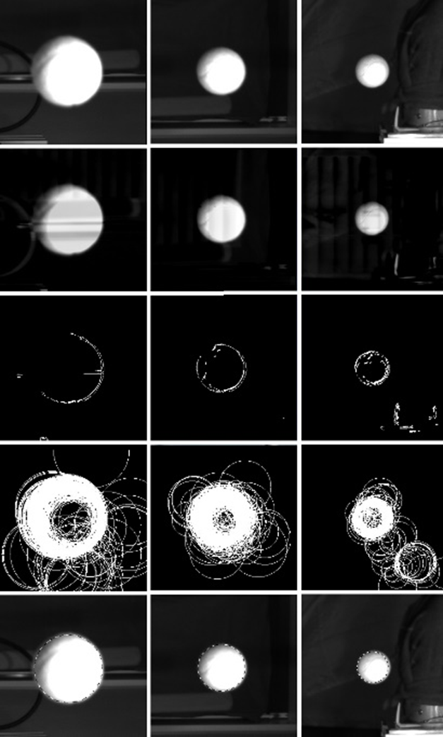Figure 1. Circle recognition with RANSAC for three images.

with the points of the boundary image. The fourth row in Figure 1 shows the hypothetical circles generated by the algorithm, and the fifth row shows the selected circle projected onto the original image.

• Stereo triangulation. This is the operation of determining spatial coordinates for the center of an object based on its pixel coordinates in two images and using camera calibration parameters.

Coordinates obtained as a result of stereo-triangulation are then transferred to the system defined as follows:

• The center of coordinates coincides with the position of the object at the time of the throw.
• One of the axes is directed vertically upwards.
• The second axis is aligned with the horizontal projection of the direction of the throw.
• The transfer of coordinates into such a system provides a two main advantages. First, three-dimensional coordinates can be replaced by two-dimensional ones. Second, approximation of the trajectory by the plane allows you to identify outliers, i.e., filter out frames on which the position of the object is measured incorrectly. Image processing errors are associated with incorrect results in the first two steps, while calibration and quantization errors affect the result of stereo triangulation. Coordinate transform is described more precisely in the end of this section.

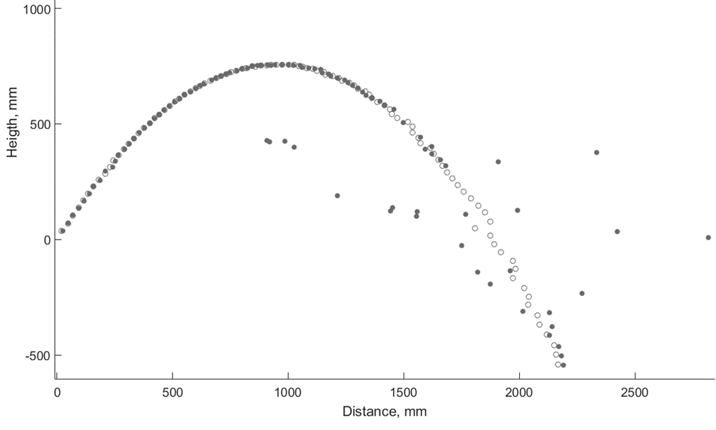Figure 2. Graph of the trajectory measured with subtraction of the background (circles) and without it (ring)

The experiments described in [27] mainly concern the theoretical assessment of positioning accuracy. In [28], the author analyzed the errors found in the real situation. This analysis is complex, since there is no true data on the position of a real object at any given time. Many errors can be detected because they distort the smoothness of the path. This curve cannot be accurately determined analytically, but it is smooth [28]. Another way to assess errors is to approximate the measured values by a simplified model of the object movement. These models are not accurate, however, if they are more accurate than the vision system, the quality of the approximation can provide information about the accuracy of the observer.

Errors of individual processing steps can be detected by visual analysis of intermediate images. The quality of border selection can be assessed by comparing the found boundaries with the boundaries of the ball on the original image. The quality of circle recognition can be estimated by projecting the circles found on the original images. For example, a visual analysis of the images in Figure 1 shows that the border detection algorithm introduces some noise, but the RANSAC assessment gives plausible results. The disadvantage of this visual analysis is that it is performed by humans and cannot transmit objective information. However, it does detect some obvious tracking errors.

Subtracting the background before running the Kenny algorithm is an optional step, but in practice, this step is necessary for correct positioning of the object at a great distance. If background subtraction is not applied, the deviations of the measured values increase significantly when the distance from the camera to the object exceeds 1.5 meters. The effect is illustrated in Figure 2. Charts are shown for the same trajectory extracted by the RANSAC algorithm with and without background subtraction. You can see that at a distance of about 1.5 meters, the measurements almost coincide, and the trajectory looks like a second-order curve. Measurements with background subtraction (rings) retain this view afterwards, but measurements without subtracting the background (circles) become chaotic. This behavior is typical of most trajectories in a dataset.

Another way to obtain more accurate data for comparison and verification is typical for RANSAC. Since RANSAC does not provide the same results for different starts, several starts give several hypotheses about the position of the ball center. A correct statistical estimate based on these hypotheses is more accurate than the result of a single run of RANSAC. The results of multiple measurements are noisy and are not supported by the model of true motion and previous statistical knowledge, for example, the probability density function. According to [35], the least squares estimate shall be used under those conditions. Such an estimate for a static parameter with unknown random noise is equal to the average measurement result. In this paper, the mean value is replaced by the median. The median and average scores give similar results, but the median score is more resistant to emissions. The median of 1000 RANSAC launches was used in compiling the training base of trajectories; a further increase in the number of launches does not change the results of the median estimate. The use of such an estimate in real time is impossible due to the large amount of computation. An existing graphics processor can perform one run of RANSAC in real time (i.e., less than 9 ms for two images and less than 1 second for the entire trajectory). It takes about 10 minutes to run the RANSAC algorithm 1000 times.

The numerical evaluation of errors is given in Table 1. Here, the coordinates extracted by a single RANSAC run are compared with the results of the median estimate for 1000 runs. Differences are considered “errors.” These numbers are not equal to real positioning errors, but they can be used to perceive the dispersion of measurements. Based on these differences, the standard deviation is calculated for each frame when the ball was thrown. In the table, each frames are combined into block to save space. Standard deviations are summarized based on 111 trajectories.

It can be seen that after the 65th frame, the parameter begins to increase strongly, and this growth is more impressive for the variant of the algorithm without subtracting the background. The reason for this increased stability at the beginning is that for the initial frames the size of the ball is larger and almost completely covers the image (compare the first and third columns in Figure 1). Therefore, the background borders make smaller distortions by the results of the border detection.

Table 1. Comparing the difference in millimeters between the measured 3D positions based on one RANSAC run and the median of 1000 RANSAC runs, for variants of the algorithm with and without background subtraction.

Frame Number	Standard Deviation		Median Error
	Without Background Subtraction	With Background Subtraction	Without Background Subtraction	With Background Subtraction
1..5	7.9	6.4	1.6	0.8
6..10	4.0	1.9	1.8	0.9
11..15	3.7	2.1	2.0	1.1
16..20	2.8	1.9	1.6	0.5
21..25	2.1	1.8	1.4	0.3
26..30	4.0	2.2	2.2	0.5
31..35	22.1	17.2	2.9	2.2
36..40	10.9	4.0	3.4	0.4
41..45	24.8	3.2	3.7	0.4
46..50	29.8	3.9	4.5	0.7
61..65	63.9	14.8	5.5	1.0
66..70	187.4	41.3	10.5	4.2
71..75	305.6	138.5	20.4	5.4
76..80	520.4	242.2	208.2	7.3
81..85	897.0	229.3	171.9	8.0
86..90	1361.6	197.5	163.9	8.4
91..95	1450.0	212.1	176.1	9.3

It can be seen that even for the option with background subtraction, the standard deviation after the 70th frame reaches very high values. Standard deviation may not be the best option, as it has low emission resistance. Therefore, columns in the right-hand part of the table show median differences for the same blocks. The median results look the same as for standard deviations, but they are more detailed. For the algorithm without background subtraction, the average error lies at 3σ interval for static spheres, estimated as 6.75 mm [26], up to the 60th frame. For the algorithm with background subtraction, this property is preserved up to the 80th frame. In the version without background subtraction, an average value of more than 20 cm is reached after the 75th frame. This means that most frames are outliers in this area. Thus, measurements without background subtraction are practically useless.

Position measurements can be divided into inliers and outliers. Outliers are defined as measurements that are completely useless, even harmful for trajectory restoring. Inliers may be wrong, but they help to improve the score. Obviously, it is not possible to determine with 100% certainty whether a measurement is an inlier or outlier. The huge difference between the standard deviation and the median error at the end of the trajectory shows that outliers make up a large proportion of the measurements.

Trajectory construction demonstrates specific properties of these errors. Figure 3 shows three graphs describing the trajectory: relationship between the height of the object and the distance from the camera (upper graph), dependence of height from the frame number (bottom left) and the dependence of distance from the frame number (bottom right). It is easy to see that the first and third graphs appear to be noisy on the right side, and the height–time dependence retains the appearance of a smooth curve of second order. In other words, errors are mainly related to distance measurement.

The reason for error localization in one dimension is that when the distance to the object exceeds the distance between the cameras of the stereo system, one pixel has a greater influence on the measurement of distance from the camera than on the measurement of other coordinates. An illustration of this property is shown in Figure 4. Experiments show that the error value at large distances is significant for tracking in terms of measuring distance. This problem can be overcome by increasing the number of cameras used for tracking, but this can be costly.

The cameras must be located so that the effect of large distance errors on the quality of the system function is minimized. The following question should be answered. In which part of the path is accurate positioning the most important? During the first experiments, the cameras were located opposite the throwing device. In this situation, positioning in the first frames is the least accurate. It was possible to accurately position the ball from the 10th or 12th frame. In further experiments, the cameras were moved to the side of the throwing device. In this case, positioning in the initial part of the trajectory is quite accurate, but the final part of the trajectory is measured with higher errors. High accuracy in the initial part of the trajectory and lower accuracy   in  the final

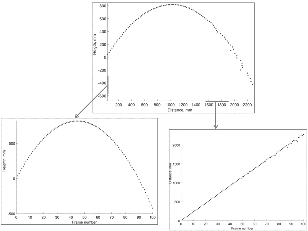Figure 3. Dependence between height of the object and distance from the camera (upper graph), dependence of height on the frame number (bottom left) and dependence of the distance on the frame number (bottom right).

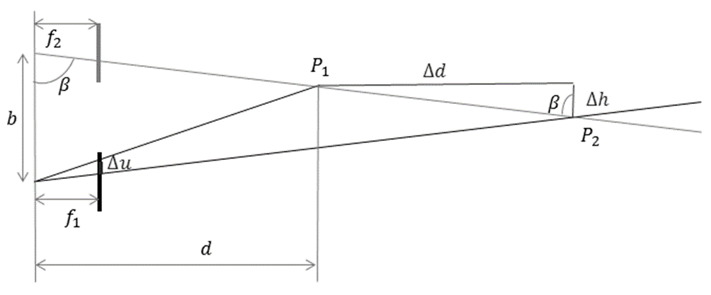Figure 4. The effect of pixel error Δu on 3D positioning errors when measuring the height Δh and the distance Δd of an object.

stage is preferable than vice versa, due to the following factor. The final part of the trajectory is not processed in real time. Under actual transportation conditions, the ball will already be in the gripping workspace. Tracking the final part of the trajectory is used only for development of a trajectory training base; therefore, its accuracy can be improved by applying 1000 runs of RANSAC to the data. Accurate positioning is necessary to measure launch parameters: speed, throw angle, position in the first frame, etc. Another factor is ball capture; the measurement of the ball position in the final region will not be accurate in any case. The robot moving in the field of view generates excessive distortions in the functioning of the algorithm. Because of these factors, the location of the camera on the side of the thrower is more likely than vice versa. It would also be possible to arrange the cameras in a different way: at a greater distance from each other or not parallel to the direction of the trajectory. However, as a result, the measurement error will not be localized in dimension coinciding with the direction of the object motion, as shown in Figure 3. In fact, this localization is very useful for correcting errors. In this measurement, the object moves at an almost constant speed, and the movement can be approximated by a second-order polynomial.

Since it is undesirable to use analytical models of object movement, approximation is applied only for the distance from the camera to the object and only at the final stage of the trajectory (starting from the 60th frame). The graph of the measured and approximated values of the distance to the object is shown in Figure 5. From a visual point of view, the results of the approximation look believable.

The stereo system used to track the trajectory of a thrown object measures its position in the coordinate system associated with the optical center of the left camera. In principle, trajectory prediction can be made in this form as well, but then the degree of trajectory proximities will be determined not only by the similarity of their shape, but also by the direction of the throw and the position of the point from which the throw is made. We have proposed to transform the coordinates of the thrown object into such a system where the trajectories can be compared and predicted based solely on the shape of the trajectory.

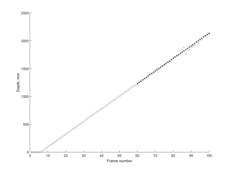Figure 5. The difference between the measured (red circles) and approximated (blue points) values of the distance to the object

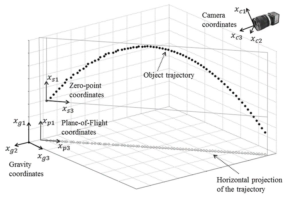Figure 6. Mutual arrangement of coordinate systems

The purpose of coordinate transformations is to present the trajectories of thrown objects in a form in which it will be convenient to compare them. For this, the following sequence of coordinate transformations is proposed:- The three-dimensional system x_c1 Ox_c2 x_c3, in which the point O coincides with the optical center of the left stereo pair camera, and the axis x_c3 is aligned with the optical axis of the camera. In this coordinate system, the position of an object is measured by the stereo pair.

– The three-dimensional system x_g1 Ox_g2 x_g3, in which the axis x_g1 is aligned with the gravity vector, and the plane formed by the other two axes is, respectively, horizontal. This coordinate system allows you to localize the effect of gravity in one spatial dimension. As will be shown below, the transfer from such a system to the x_p1  Ox_p3 flight plane is simpler than from the x_c1 Ox_c2 x_c3 system. The transition matrix from x_c1 Ox_c2 x_c3 to x_g1 Ox_g2 x_g3 is determined during stereo system calibration. The gravity vector in the x_c1 Ox_c2 x_c3 system can be determined by hanging the load on the thread: in equilibrium, the thread is parallel to the desired vector.

– The two-dimensional x_p1 Ox_p3 system (flight plane), in which the x_p1 axis is aligned with the x_g1 axis, and the horizontal projection of the object velocity lies on the x_p3 axis. In the event that lateral forces do not act in flight on the body (they can be associated, for example, with the action of the wind or with the Magnus effect), the flight path lies in such a plane. Experiments conducted in [20] showed that the influence of lateral forces on the flight of an object can be neglected. Since the real direction of the throw in each case will be different from the others, then the transition matrix between the systems will be different for each case. The two-dimensional system x_s1 Ox_s3 in which the directions of the axes coincide with those in x_p1 Ox_p3, and the center is located on one of the first points of the trajectory. Transferring the trajectory to such a coordinate system ensures result independence from the spatial location of the point from which the throw was made. An analysis of the measurement accuracy carried out in [28] showed that the accuracy in the first few frames is slightly worse than in the subsequent frames. Therefore, the sixth point on the trajectory was chosen as the common center of coordinates.

The mutual arrangement of the coordinate systems is shown in Figure 6. At the stage of predictor learning, all trajectories in the database are converted into the  x_s1 Ox_s3 system and saved in this form. In the process of predictor’s work, the current XC trajectory is converted to the x_s1 Ox_s3 system; prediction is performed in this system, and then the result YС is converted back to the original coordinate system.

This was the procedure of extracting information about tracking the thrown tennis ball. Considering more complex-shaped objects will require use of more specific image processing algorithm. The procedure of stereo triangulation will be the same, while the question of how to define pixel coordinates of the object’s center must be answered by other means instead of circle recognition. Various methods for object positioning task were developed such as rule-based algorithms, pixel-based classification, analysis of brightness distribution, convolutional neural networks, and other techniques. Development of image processing approach for complex-shaped objects is a subject of future work.

3. Predicting the trajectory of a thrown object

From the point of view of the subtask of trajectory prediction, the existing systems of robotic object capture on the fly can be divided into three groups:

• Accurate throw systems. The high accuracy of the throw (that is, the small deviation of the initial velocity and direction of flight from the given value) makes it possible to ensure that the trajectories of the thrown objects turn out to be almost identical. In this case, there is no need to predict the trajectory anew after each throw. It is enough to make a throw once, to track the trajectory of the object and to develop the trajectory of the capture device based on the results. This approach is applicable to objects with high aerodynamic stability (for example, cylindrical objects in [16]). If dropped objects do not have the required aerodynamic stability (studies in [22] and [16] show that even objects that are as simple in shape as a tennis ball and a hollow metal cylinder, respectively, do not possess it), this approach ceases to be useful.
• Interactive capture systems. In such systems, prediction is not used: movement of the capture device is determined by the current position of the object. For example, in [6], the movement of the working body is set in such a way as to maintain a constant value of the angle of view for an object in an image from a camera attached to a capture device. In [5], at each moment in time, the movement of the robot is set in the direction of the current position of the object. The implementation of such systems requires a high response speed of a robotic capture device and a high efficiency of obtaining information about object movement (for example, in [5] a vision system was used, in which the frame rate was reduced to 1 kHz by directly connecting video matrix elements to the processor). The approach is not applicable if the throw is made from a long distance and you need to choose in which area of the working space to place the gripping device (just as the football player-goalkeeper first chooses which corner to defend and then catches the ball). Since transportation of objects in an industrial environment involves throwing over a distance of several meters, this method is not suitable for such systems.
• Systems with long-term forecasting. These include the ones described in [1-4,7-11] as well as the system discussed in this section. A more detailed overview of such systems is given below.

The majority of the ballistic trajectory predictors isbased on the modeling of forces acting on the body. In the simplest case, it is assumed that the only such force is gravity (as if the body was moving in a vacuum). Such a model was considered in [2,3,7]. Prediction of the trajectory is carried out by approximation of the measured values in a parabola. In [10], the model was extended to predict the trajectory of asymmetric objects (in the experiments, empty and half-filled plastic bottles, hammers, tennis rackets and boxes were used). Prediction was made on the basis of the assumption that the acceleration vector of the object was constant over all six degrees of freedom. Strictly speaking, this assumption is wrong. The body movement under the action of gravity and air resistance is given by a differential equation which has no analytical solution and is solved in practice by numerical methods. This approach was used to predict the trajectory in a number of works [4,8,9]. Further complication of analytical models leads to a significant increase in the volume of computation [15].

On the other hand, people acquire the ability to catch thrown objects at an early age without any knowledge of aerodynamics. We catch a thrown ball based on our previous experience. Because of this, it was suggested [18,19] to use a trajectory predictor based on previous experience. In [18], a neural network predictor was proposed as a means of prediction, but it did not provide adequate forecast accuracy. Moreover, the results of prediction by neural networks are difficult to interpret; therefore, it was later proposed to apply a more transparent method of k nearest neighbors [19]. The development of individual details of this method is described in the articles of [20,21].

Here we propose the method, which lies between model-based and learning-based model. The predictor is using equations to define future positions of the object, but the parameters of these equations are obtained by the learning procedure of genetic programming. Learning does not require a sampling of past trajectories: the parameters of the model are learned from the initial part of the current trajectory. Genetic programming (proposed by Cramer [36] and developed by Koza [37]) is not a synonym of genetic algorithm. Genetic programming is an application of the principles of genetic algorithms to automatic generation of a program code. In many applications including this research genetic programming is used for generating equations, which represent the process with unknown parameters. Target program (equation) is defined as a tree consisting of nodes and arcs. The nodes are operations and the arcs are operands. Initial versions of the tree are modified via the genetic operations (mutation, crossover, selection), which are similar to the respective processes in genetics [37]. For the forecasting of trajectory, the task is to define the function for calculating future values of the coordinates based on its previous known coordinates. Genetic operations aim to define recurrent equation for trajectory forecasting. Genetic Programing OLS MATLAB toolbox was used to execute the genetic operations.

Table 2. Results of numerical experiments for 20 trajectories

#	Equation	MSE, mm
1	y(k-1) +  (-0.038706) * (x(k-1)) + (0.033084)	6
2	y(k-1) +  (-0.039329) * (x(k-1)) + (0.033553)	6
3	y(k-1) +  (-0.038554) * (x(k-1)) + (0.031962)	5
4	y(k-1) +  (-0.038689) * (x(k-1)) + (0.035645)	2
5	y(k-1) +  (-0.038774) * (x(k-1)) + (0.033805)	7
6	y(k-1) +  (-0.038546) * (x(k-1)) + (0.030245)	7
7	y(k-1) +  (-0.038526) * (x(k-1)) + (0.032994)	4
8	y(k-1) +  (-0.038740) * (x(k-1)) + (0.035160)	6
9	y(k-1) +  (-0.038601) * (x(k-1)) + (0.033345)	3
10	y(k-1) +  (-0.038454) * (x(k-1)) + (0.032473)	4
11	y(k-1) +  (-0.038388) * (x(k-1)) + (0.031648)	6
12	y(k-1) +  (-0.038501) * (x(k-1)) + (0.034544)	6
13	y(k-1) +  (-0.038134) * (x(k-1)) + (0.033116)	9
14	y(k-1) +  (-0.037313) * (x(k-1)) + (0.036494)	8
15	y(k-1) +  (-0.038036) * (x(k-1)) + (0.032546)	4
16	y(k-1) +  (-0.038347) * (x(k-1)) + (0.034728)	4
17	y(k-1) +  (-0.038149) * (x(k-1)) + (0.034948)	3
18	y(k-1) +  (-0.037972) * (x(k-1)) + (0.033884)	4
19	y(k-1) +  (-0.037583) * (x(k-1)) + (0.032284)	7
20	y(k-1) +  (-0.037841) * (x(k-1)) + (0.036221)	7

Numerical experiment on trajectory prediction was conducted using the tool [38] in two stages. On the first stage, we tried to define the common trajectory equations by learning from various trajectories. This try failed: the trajectories are different from each other and equation may be good for one trajectory and useless for another. Therefore we changed our strategy. On the second stage of experiment the initial part of each trajectory (first 50 frames) was used for learning the recurrent formula of this trajectory. Then the accuracy of this formula was checked on frames from 60 to 80. Learning procedure was applied to 20 trajectories acquired during the throwing experiments. The results are presented in table 2.

Each row shows the results for one trajectory. First column is trajectory number. The second one show equations, defining the height of the object y on frame number k as a function from its height y and distance x on previous frames. The right column show the standard deviation of the predicted ball position from the real one. It may be seen that the standard deviations of predicted height do not exceed 10 mm. According to the three-sigma rule the errors of prediction do not exceed 30 mm with high probability. All equations generated by the algorithm are relatively simple and have the same type: linear dependence from both coordinates of the previous frame. At the beginning of learning genetic operations often generate more complicated equations. These equations may include coordinate values from several previous frames.

4. Conclusion

We have proposed an algorithm for extraction and prediction of the ballistic trajectory based on video signal. Object trajectory is extracted from video sequence by the image processing algorithm, which include Canny edge detection, RANSAC circle recognition and stereo triangulation. The model of object motion is defined by the genetic programming. The result of the exploration is a recurrent formula for calculation of the object’s position. Numerical experiments with real trajectories of the thrown tennis ball showed that the algorithm is able to forecast the trajectory accurately.

1.  Gayanov, R., Mironov, K., Kurennov D.: Estimating the trajectory of a thrown object from video signal with use of genetic programming, 2017 IEEE International Symposium on Signal Processing and Information Technology (ISSPIT), Bilbao, Spain, pp. 134 to 138, December 2017.
2.  Hove, B., Slotine, J.-J.: Experiments in Robotic Catching, American Control Conference, Boston, USA, pp. 381 to 386, 1991.
3.  Nishiwaki, K., Konno, A., Nagashima, K., Inaba, M., Inoue, H.: The Humanoid Saika that Catches a Thrown Ball, IEEE International Workshop on Robot and Human Communication, Sendai, Japan, pp. 94 to 99, October 1997.
4.  Frese, U., Baeuml, B., Haidacher, S., Schreiber, G., Schaefer, I., Haehnle, M., Hirzinger, G.: On-the-Shelf Vision for a Robotic Ball Catcher, IEEE/RSJ International Conference on Intelligent Robots and Systems, ,Maui, Hawaii, USA, pp. 591 to 596, November 2001.
5.  Namiki, A., Ishikawa, M.: Robotic Catching Using a Direct Mapping from Visual Information to Motor Command, IEEE International Conference on Robotics &Automation, Taipei, Taiwan, pp. 2400 to 2405, September 2003.
6.  Mori, R., Hashimoto, K., Miyazaki, F.: Tracking and Catching of 3D Flying Target based on GAG Strategy, IEEE International Conference on Robotics 8 Automation, New Orleans, USA, pp. 5189 to 5194, April 2004..
7.  Herrejon, R., Kagami, S., Hashimoto, K.: Position Based Visual Servoing for Catching a 3-D Flying Ob-ject Using RLS Trajectory Estimation from a Mo-nocular Image Sequence, IEEE International Conference on Robotics and Biomimetics, Guilin, China, pp. 665 to 670, December 2009.
8.  Baeuml, B., Wimboeck, T., Hirzinger, G.: Kinematically Optimal Catching a Flying Ball with a Hand-Arm-System, IEEE/RSJ International Conference on Intelligent Robots and Systems, Taipei, Taiwan, pp. 2592 to 2599, October 2010.
9.  Baeuml, B., Birbach, O., Wimboeck, T., Frese, U., Dietrich, A., Hirzinger, G.: Catching Flying Balls with a Mobile Humanoid: System Overview and Design Considerations, IEEE-RAS International Conference on Humanoid Robots, Bled, Slovenia, pp. 513 to 520, October 2011.
10.  Kim, S., Shukla, A., Billard, A.: Catching Objects in Flight, IEEE Transactions on Robotics, Vol. 30, No. 5, pp. 1049 to 1065, May 2014.
11.  Cigliano P., Lippiello V., Ruggiero F., Siciliano B.: Robotic Ball Catching with an Eye-in-Hand Single-Camera System // IEEE Transactions on Control System Technology. 2015. Vol. 23. No. 5. P. 1657-1671.
12.  Frank, H., Wellerdick-Wojtasik, N., Hagebeuker, B., Novak, G., Mahlknecht, S.: Throwing Objects: a bio-inspired Approach for the Transportation of Parts, IEEE International Conference on Robotics and Biomimetics, Kunming, China, pp. 91 to 96, December 2006.
13.  Pongratz, M., Kupzog, F., Frank, H., Barteit, D.: Transport by Throwing – a bio-inspired Approach, IEEE International Conference on Industrial Informatics, Osaka, Japan, pp. 685 to 689, July 2010.
14.  Barteit, D.: Tracking of Thrown Objects, Dissertation, Faculty of Electrical Engineering, Vienna University of Technology, December 2011.
15. Pongratz, M., Pollhammer, K., Szep, A.: KOROS Initiative: Automatized Throwing and Cathcing for Material Transportation, ISoLA 2011 Workshops, pp. 136 to 143, 2012.
16. Frank, T., Janoske, U., Mittnacht, A., Schroedter, C.: Automated Throwing and Capturing of Cylinder-Shaped Objects, IEEE International Conference on Robotic and Automation, Saint Paul, Minnesota, USA, pp. 5264-5270, May 2012.
17. Pongratz, M., Mironov, K. V., Bauer F.: A soft-catching strategy for transport by throwing and catching, Vestnik UGATU, Vol. 17, No. 6(59), pp. 28 to 32, December 2013.
18.  Mironov, K. V., Pongratz, M.: Applying neural networks for prediction of flying objects trajectory Vestnik UGATU, Vol. 17, No. 6(59) pp. 33 to 37, December 2013.
19.  Mironov, K.., Pongratz, M., Dietrich, D.: Predicting the Trajectory of a Flying Body Based on Weighted Nearest Neighbors, International Work-Conference on Time Series, Granada, Spain, pp. 699 to 710, June 2014.
20.  Mironov, K., Vladimirova, I., Pongratz, M.: Processing and Forecasting the Trajectory of a Thrown Object Measured by the Stereo Vision System, IFAC International Conference on Modelling, Identification and Control in Non-Linear Systems, St.-Petersburg, Russian Federation, June 2015.
21.  Mironov K. V., Pongratz M.: Fast kNN-based Prediction for the Trajectory of a Thrown Body, 24th Mediterranean Conference on Control and Automation MED 2016. Athens, Greece. pp. 512 to 517. July 2016.
22.  Mehta, R., Alam, F., Subic, A.: Review of tennis ball aerodynamics, Sports technology review, John Wiley and Sons Asia Pte Ltd, 2008, No. 1, pp. 7 to 16, January 2008.
23.  Szeliski, R.: Computer Vision: Algorithms and Applications, Springer, September 2010
24.  Zhang, Z.: A flexible new technique for camera calibration, IEEE Transactions on Pattern Analysis and Machine Intelligence, Vol. 22, No. 11, pp. 1330 to 1334, November 2000
25.  Camera Calibration Toolbox for Matlab, http://www.vision.caltech.edu/bouguetj/calib_doc/, visited on September 18, 2018.
26.  Pongratz, M., Mironov, K. V.: Accuracy of Positioning Spherical Objects with Stereo Camera System, IEEE International Conference on Industrial Technology, Seville, Spain, pp. 1608 to 1612, March 2015.
27.  Mironov K. V.: Transport by robotic throwing and catching: Accurate stereo tracking of the spherical object, 2017 International Conference on Industrial Engineering, Applications and Manufacturing (ICIEAM).
28.  Lee, J.H., Akiyama, T., Hashimoto, H.: Study on Optimal Camera Arrangement for Positioning People in Intelligent Space, IEEE/RSJ international conference on intelligent robots and systems, Lausanne, Switzerland, pp. 220 to 225, October 2002.
29.  UI-3370CP – USB 3 Cameras – CAMERAFINDER – Products, http://en.ids-imaging.com/store/ui-3370cp.html, visited on September 25, 2014.
30.  Goetzinger, M.: Object Detection and Flightpath Prediction, Diploma Thesis, Faculty of Electrical Engineering, Vienna University of Technology, June 2015.
31.  Canny, J.: A Computational Approach to Edge De-tection, IEEE Transactions on Pattern Analysis and Machine Intelligence, Vol. 8, No. 6, November 1986.
32.  Hough, P.: A method and means for recognizing complex patterns, U.S. Patent No. 3,069,654, December 1962.
33.  Scaramuzza, D., Pagnotelli, S., Valligi, P.: Ball Detection and Predictive Ball Following Based on a Stereo-scopic Vision System, IEEE International Conference on Robotics and Automation, Barcelona, Spain, pp. 1573-1578, April 2005.
34.  Fischler, M. A., Bolles, R. C.: Random Sample Con-sensus: A Paradigm for Model Fitting with Applications to Image Analysis and Automated Cartography, Communications of the Association for Computing Machinery, Vol. 24, No. 6, pp. 381 to 395, June 1981.
35.  Hlawatsch, F.: Parameter Estimation Methods: Lecture Notes, Grafisches Zentrum HTU GmbH, Vienna, Austria, March 2012.
36. Amrouche, N., Khenchaf, A., Berkani, D: Tracking and Detecting moving weak Targets, Adv. Sci. Technol. Eng. Syst. J. 3(1), 467-471 (2018).
37.  Loussaief, S., Abdelkrim, A.: Machine Learning framework for image classification, Adv. Sci. Technol. Eng. Syst. J. 3(1), 01-10 (2018).
38.  Cramer, N. A.: A Representation for the Adaptive Generation of Simple Sequential Programs, International Conference on Genetic Algorithms and their Applications, Pittsburgh, USA, pp. 183 to 187, July 1985.
39.  Koza, J.R.: Genetic Programming: A Paradigm for Genetically Breeding Populations of Computer Programs to Solve Problems, Stanford University Computer Science Department technical report STAN-CS-90-1314, June 1990.
40.  GP-OLS MATLAB Toolbox [WebSite]. –http://www.abonyilab.com/software-and-data/gp_index/gpols, vizited on 04.09.2017.

(Click Here)

(Click Here)