1. Introduction

This paper is an extension of the article presented at the IEEE International Symposium on Signal Processing and Information Technology [1]. Initially, the problem of the rapid acquisition of an optimal route for moving the tool between processing zones on computer numerical control (CNC) equipment was considered, which is close in form to the symmetric traveling salesman problem with the Euclidean metric. For a limited number of processing zones, a solution [2, 3] belonging to the category of composite methods according to classification [4] was proposed. Construction of a convex hull, use of branch and boundary method elements, level-by-level analysis and route options design. This made it relatively easy to synthesize the optimal result for a small number of processing objects. Subsequently, the need to increase the effectiveness of this approach was revealed, where an important role, just like in the branch and boundary method, is played by a successful choice of upper bounds for the solution for which heuristic algorithms are used [5].

In the process of developing the required approximate algorithm, it was natural to use state of the art techniques from the exact method [3], while somewhat broadening the general formulation of the problem. Namely (in terms of the traveling salesman problem), to find the shortest closed route passing through n cities, visiting each city exactly once. The distance between pairs of cities is determined by a symmetric, not metric in the general case, matrix of real numbers C=||ci,j||. In [6] a natural version of the transition to the approximate method of searching for the minimum route in this formulation is presented, while the basic procedure, the basic calculation schemes and possible directions of development are described. In [7 – 9], the calculation procedures are detailed and studied, the results of testing are given, along with options for constructing the algorithm based on different schemes from the combined levels. For all benchmark tests (examples from [10] up to 100 cities inclusive, given by a complete table of distances or by Cartesian coordinates), optimal routes are obtained. Also, for all of several dozen random tests, with reported results (dimension in the range of 30-60 cities), for example, as in [11], record values of the minimum length of the route were reached, or these figures improved.

2. Basic procedure and trivial calculation scheme

If we rely on the algorithms’ classification from [12], then the level-by-level approximation (considered and tested in [7 ,9], respectively, for the matrix and coordinate representation) can be attributed to the symbiosis of “tour construction algorithms” and “monotonic algorithms for improving the tour.” Specifically, such one when the procedure for identifying improvements to the tour is involved at different levels of the multi-stage building process. According construction details, the proposed algorithm is closest to a truncated combination of three algorithms from the classification [12]. This is  C (arbitrary connection). «Let (i₁, i₂, …, i_n,) be an order of vertices. Form a two-member tour (i₁, i₂). The vertex i_l (l = 3, 4, … n) is to be included in the (l—1) -segment (pod) in such a place that the increase in the tour … is minimal». CR (most remote connection). «Act like in C. At step l (l = 3, 4, … n) in the (l—1) -st tour include the vertex i_l, for which the minimum distance to already included vertices is the largest among all vertices not yet included». CE (most economic connection). «Act like in C. At step l (l=3, 4, … n) in the (l-1) -st tour include the vertex i_l, for which the increase in the tour is minimal among all the vertices not yet included. However, this combination emphasizes somewhat different points. It should also be noted that the proposed algorithm is multi-pass. Conscious departure from the seemingly natural use of coordinates for CNC equipment should also be underscored. This is done because different metrics can be used for different types of equipment and, accordingly, of technological processes (calculations of distances between treatment zones), therefore for the sake of greater generality we will not rely on the advantages of using metric space.

The essence of the basic algorithm is as follows. Let i1, i2, …, in be a certain order of processing zones, vertices or cities in terms of the traveling salesman problem, where for definiteness i1 and i2 are the most distant cities from each other. Build a tour from i1 to i2 and back, i.e., a two-member closed tour (i1, i2, i1). Next, include the city ik (k = 3) in the existing two-member tour. This can be done in 2 ways: either (i1, ik, i2, i1) or (i1, i2, ik, i1). Since they are equivalent, we will explain the process using the first one as an example. So, for each of the two three-member tours, it is necessary to perform consecutive actions starting from the step l = 4. In step l (l = 4, 5, …, n), in each of the available (l — 1) -member tours, include one of the remaining cities il (l = 4, 5, 6, …, n) in that place of the tour, where it will provide a minimum tour increase based of the inclusion of this city. At the same time, the city of inclusion must be such that the value of the minimum increment of the tour from its inclusion is the maximum among the similar values of the minimum increments from other cities of the potential inclusion. Thus, at the last step (l = n) we obtain two complete routes. To fix one of them with the smallest length (in general, their length is the same, and the routes themselves coincide, the difference is only in the direction of the detour in the forward or reverse direction). Thus, the first of the approximate routes (Hamiltonian cycle) is obtained, which corresponds to its progenitor – a three-member tour i1, ik, i2, i1. (k = 3). Then go back to the original two-member tour (i1, i2, i1) and perform similar calculations for the remaining cities ik (k = 4, 5, … n). As the result, we will obtain n-2 approximate route options. Each route is determined by uniform constructions from its initial three-member tour i1, ik, i2, i1, (k = 3, 4, … n). We call the routes formed in this way from the original three-member tours, routes of level 0 and, for convenience, assign them indices (00, 01, 02, …) in accordance with the order of their length increase.

It can be noted that the level 00 route (s), with any significant number of cities, rarely reach optimum or are close enough to it. Therefore, it is required to continue similar constructions in order to obtain level 1 routes. They are similarly constructed for each of the n-2 initial three-member tours i1, ik, i2, i1, (k = 3, 4, … n). At the same time, at least one of the new routes (for each of k = 3, 4, … n) will be no longer by construction than its related route of level 0.

Let us explain this calculation by the example of constructing the first of the routes for level 1. In the initial tour (i1, ik, i2, i1), (k = 3), include the city im (for definiteness m = 4) alternately between pairs of adjacent cities. Accordingly, obtain three 4-membered closed tours (i1, im, ik, i2, i1), (i1, ik, im, i2, i1), (i1, ik, i2, im, i1). In step l (l = 5, 6, … n), in each of the available (l — 1) -member tours, include one of the remaining cities il (l = 5, 6, …, n) in the place of the tour where a minimum tour increase will be provided from the inclusion of this city. At the same time, the city of inclusion must be such that the value of the minimum increment of the tour from its inclusion is the maximum among the similar values of the minimum increments from other cities of the potential inclusion. Thus, at the last step (l = n) we get three complete routes. Fix one of them with the shortest length. This is the first of the approximate level 1 routes. Together with it, the initial 4-member tour is fixed as well (the value of m, k and the location of the corresponding cities in the tour).

To form the remaining routes of this level (with k = 3), we need to return to the original three-member tour (i1, ik, i2, i1) and perform similar actions with other valid values im (m = 5, 6, …, n), as in the construction of the first route of level 1. As a result, for the value of k under consideration, we obtain n-3 Hamiltonian cycles, i.e., approximate routes of level 1.

To form the remaining routes of this level (n-3 for each new k, where k = 4, 5, …, n), we need to return to the original three-member tours (i1, ik, i2, i1). Perform similar actions for each of k with admissible values of im, as in the construction of the first group of routes of level 1. As a result, for each of k (k = 4, 5, …, n) we get n-3 full routes of level 1. All received routes in each group (fixed value k) are assigned indices (10, 11, 12, …) in accordance with the order of increasing their lengths (several routes can have the same index if their lengths are equal to each other).

Similarly, routes of levels 2, 3 and subsequent are built, respectively, from 4, 5 etc. member source tours identified at the previous level.

But if nothing restricts this process, then we will have an avalanche-like growth of calculations. At the same time, when moving inward through the levels, a situation similar to the “thermal modeling” algorithms [12, 13], may be observed, where the process of improving the complete route is attenuated. For greater certainty, in [9], based on the accumulated statistical data, examples of different dimensionality of the level number, beyond which constructions are hardly advisable, are roughly indicated. When the level-by-level constructions are terminated according to the conditioned criterion, then in accordance with the multipass algorithm, we must again go to the two-member closed tour (i1, i2) for successive inclusion of the vertex ik (k = 4, 5, … n), as in the sample presented above (for the case k = 3). As a result, the route, the smallest of all constructed, is determined. It is also a potential contender for correspondence to the optimal route. This correspondence is consistently confirmed when testing the examples of a relatively small (up to 60 elements) dimension. Additionally, in practice, for achieving records from the original tripartite tours (i1, ik, i2), in tests from [10, 11, 14] with a dimension of 25-60 vertices, it was sufficient to perform calculations not for all but only for several vertices ik  where the values of index k correspond to those inclusion vertices that form zero-level routes with lower indices [7, 8]. In addition, for an overall reduction in the calculation of tests with a dimension of 60-100 vertices, extended schemes can be used, so that to reach a record we would also be limited to calculations with only lower indices from the starting extended level [9].

In general, starting from this basic procedure with a trivial calculation scheme, it is necessary to form strategies rational for practical use to create complete routes and check the criteria for stopping calculations.

3. Possible directions in organizing calculations.

First, we return to the problems of CNC machine tools. Drilling holes in printed circuit boards is one of two sources of TSP instances that are associated with practical application [16]. From an applied point of view, local search algorithms are best for solving the traveling salesman problem [17]. Nevertheless, practical problems of this kind can bring certain difficulties for local search, even with a small number of vertices. So, for example, one of such effective algorithms with the Lin-Kernigan neighborhood implemented in the Concord program [17], does an excellent job with large-dimension tests from [10], but gives, for example, a fragment of a printed circuit board with a dimension of 15 vertices, which is not an important result (approximately 103% from optimum [1]). To obtain the optimal route (Figure 1 on the right), the program needs to change the default settings, which may not help at all in more complex cases. In addition, metaheuristic methods are very popular for practical problems. [18]. They do not guarantee that the best solution to the problem will be achieved, but with a successful setup they can find a “good enough” result. Their disadvantage is the presence of a different number of control parameters [20], which makes it difficult to set up algorithms for solving specific problems.

Now let us consider possible approaches for the organization of calculations in the framework of our basic algorithm for the level-based approximation.

3.1.  Calculation on the basis of not deteriorating routes

Theoretically, each of the n-2 initial 3-member tours i1, ik, i2, i1, (k = 3, 4, …, n), from which level 1 routes are formed, can be the progenitor of the optimal route. That, however, can no longer be said about each of the 4-member (and subsequent) tours, from which routes of level 2 and further are formed. Therefore, after constructing routes of level 1 (for each of the n-2 three-member tours), the route (s) with the index zero (10) is (are) allocated to each of the received n-2 groups and the corresponding four-member tour is fixed for them, from which the subsequent construction will go (routes with a different level index and the corresponding components are not considered further). Level 2 routes are similarly constructed on this base (level 2), after which only route (s) with index zero (20) and so on is (are) also considered (that is, at subsequent levels everything related to non-zero indices routes is not participating). Thus, routes of non-zero level J (J = 2, 3, 4, …) are constructed similarly to routes of level 1, from their initial (J + 2) -fold tours, which correspond to full routes of levels (J-1) 0 . The whole process of level building can be conditionally represented by the following scheme:

• level 0_i – level 1₀ – level 2₀ … (i=0,1,2,…)

The shortest length among all level 1 routes will be the route with a zero index (level 10), which is the result of the initial embedding of a certain city iz (z ≠ 1,2, k) into a certain place of the tour (i1, ik, i2, i1). By construction, its length cannot be greater than the length of the “parent” route of level 0, resulting from embedding in the tour (i1, i2, i1) of city ik. The same applies to all derived routes with a zero index of subsequent levels, i.e., the best routes of the level cannot be longer than their ancestors. Moreover, when building at the initial levels (when moving from a lower level number to a larger number), the length of the descendant route decreases; as practice shows, this is a frequent case. However, as the level numbers increase, this happens less frequently and then fades out.

Therefore, the process of constructing routes in ascending level numbers continues, approximately as in “thermal modeling” algorithms, until a certain equilibrium is reached, understood as “no significant deviations from the found tour length are observed for a long time” [12, 13], i.e., until the termination of reducing the current length of the route. After that, the level constructions in this direction are interrupted. In the end (when the calculation is stopped in all available directions) the route is determined, the smallest of all constructed. It is also a potential contender for compliance with the optimal route. In [6, 7], the main results of testing in the framework of the considered scheme (1) for several dozens of tasks with cities given by a symmetric table of distances up to 60 objects in dimension are presented. At the same time, in all calculations, the reported record results were obtained or improved.

To explain the essence of the material presented in [1], a simple example was selected with 29 bypass objects from the TSPLIB library [10], and to demonstrate the results of innovations, a test (file xqf131.tsp) measuring 131 elements from the VLSI TSPs collection [20] created in based on SBIS data sets investigated at the University of Bonn.

Here, as a simple illustrative material, we take a classic sample containing 48 objects (att48_d.txt file) from a library with TSP data [21]. This is one of the key examples put on the cover of a famous book [22], which was used in it to illustrate existing approaches to solving the problem in question. To demonstrate the results of innovations, we will again use the same test of 131 elements.

So, let us explain the organization of the process for finding the minimum route on the selected example with 48 US cities (att48_d.txt file), given by the complete distance table. For graphical representations of the constructed routes, the Cartesian coordinates of cities from the att48.tsp [10] file will be used (in Fig.1, coordinates are on the left, and the known optimal route with a length of 33551 is on the right).

If we number the rows of the original distance table starting from 0, then the most distant cities will have numbers 3 and 16. Route level 00 (Fig. 2 upper left) built from the initial two-member tour (by cities 3, 16, 3) has a length of 34410 and a percentage ratio of 102.6% with the optimal route (hereinafter, percentages are indicated to the nearest tenth). The same figure shows the routes of level 01, level 02 (continuation of the first row of Fig. 2) and in the second row – the three longest routes of level 0 (which have the largest indices).

Sample construction 1. Route level 00 (Fig. 2 left upper) in one copy. It assumes the inclusion of the city with the number 30 in the two-member tour (3, 16, 3) (other cities with similar embedding give a greater length of the resulting route of the zero level, and, accordingly, such routes will have a larger index.

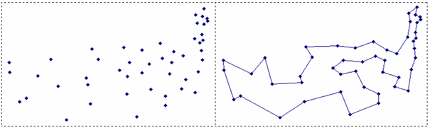Figure 1. On the left is mutual location of cities. On the right, the optimal route length of 33551.

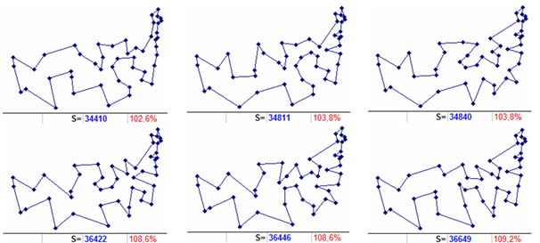Figure 2. Level 0 routes (1st row: three shortest, 2nd row: three longest). Additionally, shown are the length and deviation relative to the optimum.

The route of level 10 (00–10), built from the initial three-member tour (3, 30, 16, 3) is also one, its length is 33961 (Fig. 3 on the left). It implies embedding city 46 in the tour (3, 30, 16, 3) between cities 16 and 3.

Level 20 routes (00–10–20) are already 15, their length has not improved, and has remained the same (33961) as at the previous (parent) level 10. Each of them involves embedding one of the 15 cities: 5, 6, 7, 9, 14, 17, 18, 26, 27, 29, 34, 36, 37, 43, 44 into the initial tour in a certain place (3, 30 , 16, 46, 3). Next, for each newly formed tour routes of level 30 (00 – 10 – 20 – 30) are built, of which there are already about 152, which also do not show the change in the length of the best tour. And only at level 40 there is a decrease in length in certain directions (Fig. 3 in the center and to the right).

First, we shall consider the direction corresponding to the shorter route length (33614 Fig. 3 on the right). Let us call it “branching 1”. When building routes of level 50 from it, there will be several of them again, i.e., 22, from each of which at level 60 will be somewhere along 23-27 similar new ones, and their length does not change (it remains equal to 33614). The situation is similar at the level of 70 and 80. That is, there is a circumstance that “for a long time no changes are observed” of the lengths of routes with zero indices and therefore it is necessary to stop further constructions in this direction.

For the future, we should agree on the criteria for stopping calculations in the current direction. Let it be, for example, the following: “threefold repetition of the route length value with a zero index during the transition from level to level in the process of forming hereditary directions».

That is, in our case, calculations for this direction (branching 1) should be stopped after the formation of level 70 routes, despite the fact that we would reach the optimum (length of the route is 33551 cm. Fig. 1) already while calculating from level 90, continuing calculations for this direction. For example, when calculating from the initial closed tour 3, 1, 33, 7, 30, 16, 32, 19, 46, 31, 4, 3 (when you include city 40 between cities 33 and 7). Or from another source tour 3, 1, 33, 40, 7, 30, 16, 32, 46, 31, 4, 3 (with the inclusion of the city 19 between cities 32 and 46).

Let us now consider the second direction (“branching 2”), corresponding to the greater length of the route (33741 Fig. 3 in the center). When building from it, 4 routes of level 50 are obtained with a length that has changed to a value of 33614. From each of the corresponding four routes, the eight-member initial tours are obtained at level of 60, with about 21-24 new routes in them, while their length does not change (it remains equal to 33614). At level 70, another average of 23 routes is added. This is about 4 * 232 new calculation directions in grand total. And if during the formation of the level 80 routes there is no change in the length of at least one of them, then, according to the entered criterion, the calculations in this direction (“branching 2”) should be stopped, and therefore, in general, the entire “parent” direction of level 00 should cease. However, in reality this does not happen. When forming routes of level 80 from the initial closed tour 3, 40, 2, 8, 7, 30, 6, 16, 46, 3 (when you include city 32 between cities 16 and 46 – constructing at level 70), a route of length 33551 (Fig 1) results, which is an optimal one.

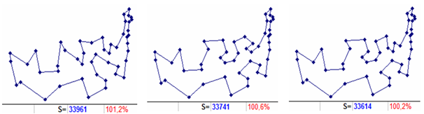Figure 3. Route of level 10 (left), and of level 40 (center and right). Additionally shown are the length and deviation relative to the optimum.

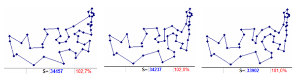Figure 4. Routes from 024: level 10 (left), level 20 (center), level 30 (right). Additionally, the length and deviation relative to the optimum are listed.

Despite the fact that the result within the declared scheme (1) has been achieved, we will continue our constructions from the 0i (i ≠ 0) levels in order to identify less labor-intensive directions. And such options are, for example, the following ones.

Sample of construction 2. Here, the optimum is reached virtually without branching after calculations at level 3₀, within the framework of the scheme (0₂₄ – 1₀ – 2₀ – 3₀). In this case, calculation starts from almost the least long (36422) route of level 0₂₄ (in Fig. 2, the bottom left). This route is one copy. It assumes the inclusion in the two-member tour (3, 16, 3) of the city with the number 32. There are three routes of level 1₀ (0₂₄ – 1₀), constructed from the original three-member tour (3, 32, 16, 3), their length is 34457 (Fig. 4 left). They suggest embedding in the tour (3, 32, 16, 3) cities 10, 19 or 34 between cities 16 and 3.

We will begin further constructions from city 10 (having a smaller sequence number). When calculating from the tour (3, 32, 16, 10, 3), the only route of level 20 is 34237 long (Fig. 4 in the center). It assumes embedding in the tour (3, 32, 16, 10, 3) city 43 between cities 16 and 10. By performing this operation, we also get a single route of level 30 with a length of 33902 (Fig. 4 on the right). This, in turn, is assuming that the only embedding in the tour (3, 32, 16, 43, 10, 3) shall be city 22 between cities 3 and 10. This embedding, in turn, results in obtaining an optimal route of length 33551 (Fig. 1). As a result, the entire calculation is significantly less time consuming than the calculations from level 00 in sample construction 1. The remaining two branches (those from cities 19 and 34) are more computationally expensive.

Here we shall note that it is possible to dramatically increase the number of ways to build optimal routes through the use of extended schemes for non-deteriorating routes.

In [8] it was shown that within the framework of the scheme (1), as a rule, there are quite a few options for constructing optimal routes; however, in some cases it is not possible to quickly reach the optimal result, therefore in [7], alternatively, extended schemes are proposed. They allow, for example, in problems with a dimension of up to 50 elements, to obtain an optimum often even at the initial state. Either they open new directions in which the optimal result is achieved in the absence of significant branching of the process, or at earlier than in scheme levels (1), which may already be more relevant for tasks in the range of dimensions, from 50 to 100 elements [9].

The first version of the extended calculation scheme:

• level (0 – 1)_i– level 2₀ – level 3₀… (i=0,1,2,…)

Here, level (0 – 1) represents some combination of level 0 and level 1 from the previous scheme. Full routes (Hamiltonian cycles) from level 0 are not built, and each of the n-2 source 3-member tours i1, ik, i2, i1, (k = 3, 4, …, n) is converted into 3 four-member one, from which the full routes are already formed from the combined level (0-1). Here, they are presented in the number of (n 2) * (n 3) * 3, which is a broader basis for the formation of full routes of levels 20 and subsequent levels. At the same time, within the framework of the scheme (1) for the formation of level 20 routes, there is, as practice shows, in all directions (n 2) or several more closed source routes, that is, a small subset of the analog from the scheme (2).

Let us explain the scheme (2) in our current example. Among the many variants of the initial routes corresponding to the level (0 – 1) i, we take two (with some average level indicators of the full route length) and at the same time non-existent (unrealizable) within the framework of the scheme (1).

Sample of construction 3. Let the first of them be the original route that implies embedding into a two-member tour 3, 16, 3 pairs of cities 15 and 30 between cities 3 and 16. As a result, we have tour 3, 15, 30, 16, 3, and the only route from it is on level 20, involving the incorporation of city 37 between cities 30 and 15, with a total length 34410, corresponding to the upper left in Fig. 2

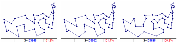Figure 5. Intermediate routes of level 30 (left), level 40 (center), level 50 (right) as part of the implementation of the scheme (2). Additionally, the length and deviation relative to the optimum are shown.

In turn, it builds only one next-level route with a zero index (level 30), with an estimated integration of city 10 between cities 15 and 37 on tour 3, 15, 37, 30, 16, 3 with the result (length 33948) indicated in Fig. 5 left. Already from this position is also obtained the only route of level 40 with the expected inclusion of city 25 between cities 3 and 15 in tour 3, 15, 10, 37, 30, 16, 3, and with length of 33932 (Fig. 5 in the center). Further, the route of level 50 is also created in a single copy indicating the inclusion of city 12 between cities 15 and 10 in tour 3, 25, 15, 10, 37, 30, 16, 3, and with length of route 33628 (Fig. 5 on the right). And already from that, after the implementation of the specified inclusion, we immediately get the optimal route (Fig. 1 on the right). As a result, all transitions from the initial to the last level pass without a single branching in the process of construction.

Sample of construction 4. Let us take, as the second similar initial tour, a route with a supposed embedding in the two-member tour 3, 16, 3 pairs of cities 22 and 30 between cities 3 and 16. There is also no corresponding route within scheme (1), since embedding from level 1 with city 22 in the case of constructions from level 00 (or with city 30 in case of constructions from level 025) will have an index number of level 1 greater than 0, which is beyond the scope of the scheme. Within the framework of scheme (2), the corresponding full routes exist and coincide, their length is 35935 (Fig. 6, left). The calculation from tour 3, 22, 30, 16, 3 gives a single route of level 20, which implies embedding city 11 between cities 22 and 30 with a full route 34694, corresponding to the central route in Fig. 6. There are already two level 30 routes (Fig. 6 on the right), they suggest embedding cities 32 or 45 between cities 3 and 16 in tour 3, 22, 11, 30, 16, 3. Both routes with the specified embedding lead to an optimal result (Fig. 1 right).

Sample of construction 5. It is also possible to note the possibility of obtaining an optimum according to the scheme (2) among the directions existing within the framework of the scheme (1), but “rejected” by the criterion of stopping the calculations. For example, in the framework of scheme (1), according to this criterion, constructions are rejected from the direction (06–10–20–30) because of the fourfold construction at each level of the same complete route. Namely, the sequential inclusion in the two-member tour 3, 16, 3 the city 43 (3, 43, 16, 3), then the city 10 (3, 10, 43, 16, 3). After that, city 40 (3, 40, 10, 43, 16, 3) and finally, city 0 (3, 40, 10, 0, 43, 16, 3), each time they build the same full length route 33633 (100, 2% of the optimum of Fig. 7, in the center). In fact, there is a threefold repetition of the length of the route and, according to the criterion, the calculation stops.

If such constructions are carried out within the framework of the scheme (0 – 1) i – 20 – 30, then the same route will be obtained 3 times in a row, which means we have only 2 repetitions, and therefore it is possible to carry out constructions at level 40 without violating the stopping criterion. And here there are already several options for obtaining the optimal route, for example, including the city 33 (3, 33, 40, 10, 0, 43, 16, 3) in the above described tour. Or for other inclusions in the framework of this scheme for other branches: (3, 33, 40, 10, 8, 43, 16, 3), (3, 40, 22, 10, 43, 16, 9, 3), (3, 40, 22, 10, 43, 16, 19, 3).

Let us present another extended scheme similar to (2), but with three levels combined.

• level (0 – 1– 2)_i– level 3₀ – level 4₀… (i=0,1,2,…)

It provides even greater opportunities for obtaining record-breaking results due to the impressive “re-selection” component of the combined entry level. (0 – 1 – 2)_i.

Sample of construction 6. So, for example, thanks to such a scheme, from tour 3, 12, 10, 43, 16, 3 (which corresponds to the construction from the combined level (0 – 1 – 2)) in our current example of 48 cities, we immediately get the optimal route. This tour is not the only one on the level combined by the scheme (3).

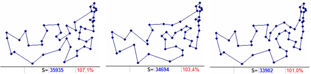Figure 6. Intermediate routes of the “combined” level (0-1) i (left), level 20 (center), level 30 (right) as part of the implementation of the scheme (2). Additionally, the length and deviation relative to the optimum are shown.

3.2.  Calculation based of the scheme with permissible deterioration of routes

Such a scheme is designed to provide flexibility in achieving record routes. This is a way to improve from a slightly worse calculation position (which is longer than the best route of the current level), which at the next or later levels can lead to a change in the current minimum in the considered direction of calculation. It is significant that this allows to avoid the situation “for a long time, no deviations from the found tour length are observed”. This approach is implemented based on the use of index variation not only as previously at the zero level, but also at subsequent levels of construction. That is, in the general case, the calculation scheme can be as follows [16]:

• level 0_i0 – level 1_i1 – level 2_i2 … (i0, i1, i2, …=0,1,2, …)

The total number of calculations here is much larger relative to the scheme (1). Therefore, from a practical point of view, one should artificially limit the potential excessive growth of the level-by-level calculations. And from this position, it is more expedient to introduce into (4) additional restrictions or to use some hybrid variants from schemes (1) – (3) and (4), for example let us consider the scheme (5), which is defined by the next three paragraphs.

If at the levels of J0, where J = 1,2,3 …, only one route is observed (with index 0), then further constructions lead only from the initial (J + 2) -member tour for it, i.e., according to scheme (1).

If there are several routes with index 0, then further constructions will lead not only from the initial (J + 2) -member tours for them, but also from all other (J + 2) -member tours that are initial for the level routes with corresponding non-zero indices, i.e., as in scheme (4).

Moreover, in order to reduce computations, directions of calculations from non-zero indices, for constructions from which the full route with a zero index of the next level coincides with the parent route (that is, in the absence of a decrease in the length), shall not be considered,).

To illustrate the scheme with permissible degradations of routes, we turn to the already considered version of the calculation from construction sample 1, where for the first time instead of one, in the direction of 20 (in the direction 00 – 10 – 20), 15 routes appear with a zero index and not improved length of 33961 (Fig. 3 left). This is just the reason to use the scheme (5).

Sample of construction 7. So, we shall start constructing routes of the 3rd level. Embedding in a certain place of the initial tour (3, 30, 16, 46, 3) each of the identified cities corresponding to the level 2 zero index does not change the generated routes of the next level with the zero index (see construction pattern 1, level 30). According to the adopted scheme, we will construct from non-zero level indices. So embedding of city 15 between cities 3 and 30 (corresponding to the route with the last, i.e., the largest index of level 2 with an initial length of 35582) results in two routes of level 30 with a decrease in length to 33614.

Further, from the first of these routes, through the implementation of the supposed embedding of city 33 between cities 3 and 15 (on tour 3, 15, 30, 16, 46, 3), 25 routes of level 40 are obtained. In one of them, the embedding of city 32 between cities 16 and 46 (in tour 3, 33, 15, 30, 16, 46, 3) allows to obtain the optimal route which is several levels earlier than indicated in construction sample 1.

From the second route, an optimal tour is also obtained, but it is built one level further.

Sample of construction 8. A stronger result is obtained when constructing from level 06, where there is (before the start of the intended embedding of city 43 in the two-member tour 3, 16, 3 ) a full route (Fig. 7, left) 35143 in length. The route of level 10 from the implementation of such embedding is one, with length of 33633 (Fig. 7, in the center) and it involves embedding the city 10 between 3 and 43 (on tour 3, 43, 16, 3). When implementing it, we already get 10 level 20 routes and, according to scheme (5), along with them, it is possible to conduct calculations also from levels 2i (where i ≠ 0). As a result of the calculation from level 27 (where the full route 34479 in Fig. 7 is on the right), when the city 22 is embedded between 3 and 10 (in tour 3, 10, 43, 16, 3), we immediately get the optimal route (Fig. 1 on the right).

It can be noted that in a similar way and with the same laboriousness (when building from level 2), optimum is obtained when calculating from the starting level 012 (the full potential route is no longer than 35808), with an estimated only integration of city 10 into the two-member tour 3, 16, 3.

4. Natural innovation in the basic calculation procedure

Having considered the main directions of calculations, and based on the statistics of the calculations carried out earlier [7–9, 16], we can draw some conclusions. For the considered possible directions of calculations in various test examples with dimensions up to 100 and a little more elements, it is always possible to obtain the optimal result with varying degrees of complexity. In this case, the optimum for each of the possible calculation schemes, as a rule, is achieved  in  many  different  ways. The  least  laborious  route

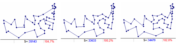Figure 7. Routes corresponding to the constructions according to the scheme (5): level 06 (left), level 06-10 (center), level 06-10-27 (right). Additionally, the length and deviation relative to the optimum are shown.

(when comparing calculations from level 0 starting tours) was often the one where the optimal route is built at earlier levels. Less often – at later levels, but in the absence of a large number of branches. The results of experiments [7–9, 16] also show the following. The more extensive the base of the starting (initial) level, as is the case with the use of advanced schemes, the higher the probability of an “earlier” approach to optimum in individual calculations from starting tours. The total number of such exits is also growing.

There is a natural opportunity to significantly increase the number of zero level starting tours from the current n-2 options within the framework of the scheme (1). That will also increase the number of corresponding approximate level routes. The essence of such an extension is as follows. For convenience and certainty, the baseline calculation procedure used the directive choice of the first two cities (maximum distance from each other). From this pair, all subsequent constructions were carried out. If calculations would be carried out from each unique pair of source cities, then the number of starting two-member tours increases to n * (n-1) / 2, where n is the number of cities. Let us return to current example (48 cities) to clarify application of new starting conditions.

Samples of construction 9. In practice, probably, such a large number (in our new conditions 1128) of initial tours is not necessary. Let us see what happens if we restrict ourselves, for example, to considering only a few starting two-member tours, from which when forming routes of the zero level we get the smallest routes with zero index (i.e., the smallest among all possible routes of levels 00).

In our example, there are only 68 (out of 1128) two-member tours with a minimum route (at level 00) of a length of 33614 (as in Fig. 3 on the right). By constructing according to scheme (1), we will reveal among them those two-member tours, from which the optimal route will be constructed at the nearest of the subsequent levels, and accordingly the number of this level. Thus, directly from all possible three-member tours, being built from each of the 68 two-member tours, the optimal route is not immediately reached. But for the individual subsequent four-member tours the optimal route (Fig. 1 on the right) is already calculated. That corresponds to the constructions from level 10. The code of these constructions, corresponding to scheme (1), is contained in table 1; it indicates the sequence of obtaining the optimal route (length 33551).

Table 2 contains similar information, but this time from a small sample of the remaining starting two-member tours. In it, the best routes of zero levels (routes of level 00) exceed the minimum length of 33614 (that is, more than the tours from the previous table). The corresponding constructions for each of those two-member tours of scheme (1) also lead to the identification of the optimal route, with the implementation of inclusion from level 10.

The above tabular data suggests that there are no clear preferences when choosing a two-element tour from the available starting conditions in order to obtain a “short” calculation of the optimal route. For example, our initial starting two-member tour (3 16 3) from the most distant cities is with index 75 according to the criterion for the route length of level 00 almost exactly in the middle of the totality of 1,128 two-member tours (among the sequence numbers in ascending order from 532 to 574). From the point of view of building an optimal route (sample of building 1 – 8), it is not very fast relative to others. But the starting two-member tour 12 38 12 with the sequence number 1127 (Table 2 last line) with the length of the 00 level route equal to 35400 (Fig. 8 on the left) is almost perfect from the same point of view (like some others presented in both Tables).

And this is despite the fact that its starting indicators are next to the last ones in proximity to the optimum length of its best route among all 1128 results of levels 00. However, the optimal path is quickly and unequivocally (without a single branching) built from level 03 (basic length 35659 in Fig. 8 in the center). Specifically, first begins the inclusion in the two-member tour of the city 28 (12 28 38 12). As a result, a route with the length of 34603 is built (Fig. 8 on the right). Then, the only possible inclusion of the next level 10 is the insertion of city 32 (12 32 28 38 12) and, as a result, the already known optimal route is obtained (Fig. 1 on the right).

Table 1: Sequential Data

The sequence number of the original tour	The order of the cities for the starting two-member tour	The length of the level 0i tour(at the beginning of the direction for constructing the optimal route)	Order of cities of a three-member tour (level 0i)	Length of a tour of level 10	Order of cities in a four-member tour, directly from which the optimal route is built (level 10)
3	1 30 1	35374 34110	1 12 30 1 1 15 30 1	33628 33628	1 15 12 30 1 ––– // –––
8	1 43 1	35137 35131	1 22 43 1 1 24 43 1	33879 33879	1 22 24 43 1 ––– // –––
22	6 37 6	34947 35613	6 22 37 6 6 24 37 6	33955 33955	6 22 24 37 6 ––– // –––
39	17 37 17	35191	17 24 37 17	33955	17 22 24 37 17
45	22 27 22	34483	22 24 27 22	33955	22 24 37 27 22
53	27 37 27	34704 35769	27 12 37 27 27 24 37 27	34701 33955	27 28 12 37 27 27 22 24 37 27

Table 2: Tour Measurements

Tour Number	Order of starting cities according to the scheme (1) tour	Index among all tours of levels 00	Tour length of level 00	Tour length of level 0i (starting to calculate)	Order of three-member tour cities (level 0i)	Tour length of level 10
69	3 10 3	1	33633	35877	3 22 10 3	34479
70	3 43 3	1	33633	35254	3 22 43 3	34479
331	24 38 24	33	34151	35539 36239	24 21 38 24 24 40 38 24	34668 34151
332	24 43 24	33	34151	35131 35420 36138 35880	24 1 43 24 24 8 43 24 24 22 43 24 24 40 43 24	33879 33985 33879 34151
333	38 43 38	33	34151	36575	38 22 43 38	34510
394	22 24 22	46	34276	35881 35128 35561 36138 34483 36885 36138	22 1 24 22 22 6 24 22 22 8 24 22 22 17 24 22 22 27 24 22 22 37 24 22 22 43 24 22	33879 33955 33985 33955 33955 33955 33879
639	22 43 22	90	34479	36427 35137 35254 35818 36152 36138 37297	22 0 43 22 22 1 43 22 22 3 43 22 22 9 43 22 22 20 43 22 22 24 43 22 22 38 43 22	33991 33879 34479 33991 34094 33879 34510
854	10 22 10	156	34755	35877 35022	10 3 22 10 10 28 22 10	34479 34094
1127	12 38 12	258	35400	35659	12 28 38 12	34603

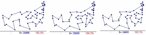Figure 8. Routes from the starting cities 12 and 38 corresponding to the constructions according to the scheme (1): level 00 (left), level 03 (center), level 03 – 10 (right). Additionally, the length and deviation relative to the optimum are shown.

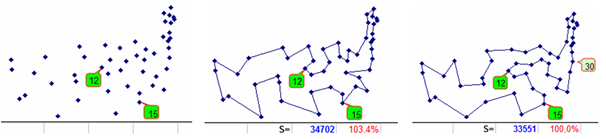Figure 9. Cities 12 and 15 that make up the starting two-member tour (left). The route of level 00, corresponding to the constructions according to scheme (1), implies the inclusion of city 30 (in the center). Route level 00 – 10 (right), resulting from the inclusion of the city 30 (optimal). Additionally, the length and deviation relative to the optimum are shown.

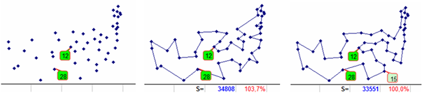Figure 10. Cities 12 and 28 constituting the starting two-member tour (left). The route level 00, corresponding to the constructions according to scheme (1), implies the inclusion of the city 15 (in the center). Route level 00 – 10 (right), obtained as a result of the inclusion of the city 15 (optimal). Additionally, the length and deviation relative to the optimum are shown.

Samples of construction 10. It is necessary to separately distinguish the group of constructions where the optimal tour is obtained at the earliest stage (from the beginning of the calculations) when implementing the inclusion in the starting two-member tour of the third city, i.e., after calculations at the zero level.

Fig. 9 (left) shows an illustration of the starting conditions for the calculation of a two-member tour between cities 12 and 15. In the center of this figure, the shortest route (length 34702) is being built for those cities which have a zero level route (level 00). It is the only one and involves the inclusion in the two-member tour of the city 30. After the realization of this inclusion, we obtain the optimal route Fig. 9 (right).

Also, when implementing the inclusion of level 00, an optimal route is constructed from a two-member tour between cities 12 and 28. Fig. 10 (left) is an illustration of the starting calculation conditions for this two-member tour. In the center of the figure, the shortest (length 34808) zero level route (level 00) is shown. There are two such routes and, accordingly, two directions of construction according to the scheme (1). The first one, which implies the inclusion of city 2, is a dead end one for reaching the optimum. The second one, which implies the inclusion of the city 15, after its implementation immediately builds the optimal route Fig. 10 (right).

For more commonality, Fig. 11 shows 4 more routes of the zero level from binomial tours, but with a non-zero index (levels 0i, i ≠ 0: the first row in the center and to the right, the second row in the center and to the left). Each of the directions corresponding to them, after the implementation of the proper inclusion of the third city in the corresponding route of the two-member tour, also immediately leads to an optimal result (Fig. 11, second row rightmost). This happens again when constructing from the zero level, but only already when implementing the inclusion corresponding to a non-zero index (from the level 0i, i ≠ 0).

Unfortunately, in the absence of a general criterion for choosing the “correct” pairs of starting two-member tours, in order to identify all three-member tours, from which the optimal route is immediately constructed, 17296 possible options will have to be considered (in general, n * (n-1) * (n-2 ) / 6, where n is the dimension of the problem).

5. Features of finding the best route in tasks with a large dimension

In the light of the innovations outlined in the previous section, at the very beginning, there emerges a very large number of directions of calculations from each of which it is potentially possible to get the best route.

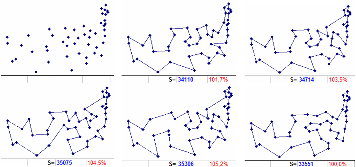Figure 11. The mutual position of 48 cities (upper left). The optimal route is 33551 long (bottom right). The rest: routes of level 0i, directly transformed after the inclusion of the corresponding third city in the optimal route. Additionally, the length and deviation relative to the optimum are shown.

In such examples as ours (dimensionality of 48 cities) and even twice as large dimensionality, it is still possible to authorize the definition of not only the best route, but also the youngest level where it is reached (along with a full set of options for building it on it). This was shown in construction samples 10.

For examples with a dimension somewhat greater than 100 elements, such an approach (i.e., the calculation of “breadth”) is already quite laborious. Therefore, we first denote a simplified version of the organization of calculations among the set of initial two-member tours. For each unique pair of source cities, determine the minimum route of level 00, and the corresponding city for inclusion in the two-member tour (if there are several, then one of them). Index all (n * (n-1) / 2) obtained routes in order of increasing length (we call these indices global). Limit the number of calculations from starting two-member tours (or groups of tours) only to those of them that have small global indices.

In addition, we will somewhat limit the number of calculations in scheme (5). One of its possible modifications can be formulated as the scheme (6) determined by the next paragraph.

If at the levels of J0, where J = 1,2,3 …, only one route is observed (with index 0), then further constructions will only lead from the initial (J + 2) -member tour, i.e., according to the scheme (1).If there are several routes with index 0, then further constructions will lead not only from the initial (J + 2) -member tours for them, but also from all other (J + 2) -member tours that are initial for the level routes with corresponding non-zero indices, i.e., as in the scheme (4). At the same time, in order to further reduce the computations, as compared with scheme (5), we shall consider only separate directions of calculations from non-zero indices of the current level (“current-baseline”). These are the directions from which a chain of routes with zero indices of subsequent levels with decreasing lengths is built without branching. Moreover, the length at the end of the chain (before branching occurs), even if only one link actually turns out, should be less (or at least not more) than the length of the route with zero index of the “current-base” level.

Let us consider how this is implemented using the example of calculation, for a test with a dimension of 131 elements (Fig. 12, top row to the left) from the ASIC data set of the VLSI TSP collection (file xqf131.tsp) [20]. For convenience, we will use the numbering of the test elements (in this case, vertices or points) defined by a set of Cartesian coordinates, starting from 0 (and not from 1, as in the original source [20]).

Sample of construction 11 (from a two-member tour with the global index of 0). Among the routes of level 00, constructed from all possible combinations of initial two-member tours, the shortest length is 580.23 (Fig. 12 upper row in the center – for simplicity, we shall ignore digits after hundredths) and, accordingly, two of them have a global index of 0. The first one combines the vertices 28 66 and the second one has the vertices 28 62. Both assume that vertex 111 is included in the initial tour. Let us consider the constructions from the first one.

Thus, from the three-member tour (28 111 66 28) a minimum route is built (Fig. 12 upper row to the right) with a length of 579.99. It predetermines 3 variants of the inclusion vertices (25, 26 or 18) corresponding to the zero level index, and therefore along with them, according to scheme (6), other remaining vertices of the possible inclusion should be considered. Among all the directions, the inclusion of the vertex 34 (28 34 111 66 28) seems to be one of the most promising for further development. After it, a diminishing chain of lengths for complete routes is constructed with zero indexes of subsequent levels up to level 5, where there are three routes with zero index length 574.77 (Fig. 12 bottom row to the left) again. Therefore, the condition of the scheme (6) for the final length of the chain is less than the length of the route with the zero index (579.99) of the “current-base” level. Since then there are three inclusions (from zero level indices) into a seven-member tour (28 34 97 111 106 96 66 28), all remaining vertices with nonzero indices should also be considered. At this stage, there is a good potential for the development of directions at the inclusion vertices with zero indices (60 94 and 95). Consider the first of them – the inclusion of vertex 60 (28 34 97 111 106 96 60 66 28), from which a sequence of decreasing routes  to  level  8   is   unambiguously   constructed,   where  36

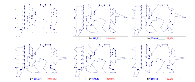Figure 12. The mutual position of 131 points (top left). Record route length 566,42 (bottom right). The rest: a sequence of key intermediate routes. Additionally, the length and deviation relative to the record are shown.

directions (vertices) characterizing routes with a length of 571.17 with a zero index appear (Fig. 12 bottom row in the center). Any of them does not reduce the length of the route with a zero index on the next level. But from one of them – from the inclusion of vertex 93 in the ten-member tour (28 34 11 93 97 111 106 79 79 60 66 28), 44 more routes are formed with a zero index and with the same length. And here already (when constructing routes of the next level), a record 566.42 length is not improved (Fig. 12 bottom row to the right), from the inclusion of vertices corresponding to non-zero level indices. This happens when vertices 77, 87 (correspondence to index 4) or 13 (correspondence to index 9) are included between vertices 11 93 in tour 28 34 11 93 97 111 106 96 79 60 66 28.

Here is the record tour: 66 62 57 58 59 60 72 71 79 78 82 83 84 85 89 90 94 95 96 103 102 110 109 108 114 118 115 119 116 121 128 127 126 130 125 124 123 112 107 106 105 101 100 99 104 113 117 120 129 122 111 97 88 92 98 93 91 87 86 81 80 77 76 74 67 63 73 52 44 25 26 18 24 16 15 14 13 17 12 4 11 5 0 6 7 1 2 8 9 3 10 23 43 42 41 40 39 22 38 37 36 21 35 34 33 20 32 31 30 19 29 28 27 45 53 54 46 47 48 49 50 51 56 55 61 64 68 65 69 75 70 66.

It is achieved according to the scheme (6), at constructions from level 9 (00 – 163 – 20 – 30 – 40 – 50 – 60 – 70 – 80 – 9i, где i=4, 9), which is two levels earlier than at calculation according to scheme (5) from a two-member tour with the most distant cities in [15]. If the optimal route stated in [20] is calculated with an accuracy that is used in applied calculations for CNC (conventionally with “computer” accuracy), then we obtain the length 567.20, i.e. Our record route was shorter. In the integer metric used in [20], our route will be one unit longer.

Sample of construction 12. Let us check whether the path of obtaining a record result in certain areas will be shorter if we use scheme (1) for calculations from the same two-member tour with a global index of 0, as in construction 11.

And this direction is found. Let us consider the same two-member tour which unites the vertices of 28 66, but with the vertex of embedding 34, which in the framework of scheme (1) corresponds to the construction from level 084 with a route of 630.94 in length (Fig. 13 on the left).

From it, there are unambiguous constructions of improving routes with zero indices of subsequent levels up to the formation of routes of level 5. Where it appears after being included in the six-membered tour of vertex 11 (28 34 11 13 80 86 66 28), 33 routes with zero index that duplicate the route of level 40 (Fig. 13 in the center).

From it, there are unambiguous constructions of improving routes with zero indices of subsequent levels up to the formation of routes of level 5. Where appear, after being included in the six-membered tour of vertex 11 (28 34 11 13 80 86 66 28), 33 routes with zero index that duplicate the route of level 40 (Fig. 13 in the center).

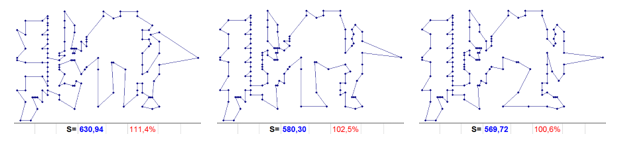Figure 13. The sequence of key intermediate routes. Additionally, the length and deviation relative to the record are shown.

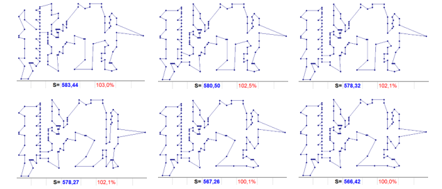Figure 14. The sequence of key intermediate routes leading to the record. Additionally, the length and deviation relative to the record are shown.

From one of them (as a result of consecutive unambiguous inclusions in the seven-member tour 28 34 11 13 80 86 66 28 vertices 122 106 102), a chain of routes with zero indices of subsequent levels with a minimum length of the resulting route equal to 569.72 is built without branching (Fig. 13 on right). Moreover, there are two such routes and two new directions respectively from the inclusion of vertices 100 and 99 (28 34 11 13 80 86 122 100 106 102 66 28 – the first, and 28 34 11 13 80 86 122 99 106 102 66 28 – the second). Both directions, in order to reach the record route with a length of 566.42 (Fig. 12 bottom row to the right) assume that the 75 vertex is definitely turned on between 28 and 66, and at the next level 100 – alternative inclusions of the vertex 108 (between 102 and 106).

Sample of construction 13. The record route can be calculated at earlier levels by a repeated number of times and also according to a less laborious scheme (1), if not limited to the calculation, only from the global zero index.

So, for example, among the routes built from all possible combinations of the original two-member tours, the route from the two-member 6 6 6 6 level 00 with a length of 583.44 (Fig. 14 at the top left) has a global index of 16. It alone determines the inclusion of the 87 in the two-member tour.

Then, there is an unambiguous inclusion in the three-member tour of the vertex 54 (6 87 89 54 6), after which 9 routes appear with the index 0 level 2 with a length of 580.50 (Fig. 14 in the center above). Among the corresponding vertices of inclusion, only embedding vertices 4 and 112 reduce the route to the next level. Let us track the first of them (6 4 87 89 54 6).

From it, there is an unambiguous reduction in the length of the routes to the formation of tours of level 5, where 8 routes appear with the index 0, length 578.32 (Fig. 14 at the top right). The corresponding embedding in each of the tours of level 50 again multiplies routes with index 0 of the next level (an average of 8 routes without a change in length). And only embedding already in one of the many tours of level 60 leads to a decrease in the length of the route of level 70 to 578.27 (Fig. 14 at the bottom left).

This reduced route resulted from the inclusion of the vertex 88 in the eight-membered tour (6 0 11 4 87 88 97 89 54 6). The constructed route predetermines three possible embeddings in the tour 6 0 11 4 87 88 97 89 54 6 peaks 98 93 or 91.

Each of these inclusions gives a new reduced route with a length of 567.26 (Fig. 14 in the center below), and, accordingly, 3 initial tours with a unique inclusion of vertex 106. This inclusion in any of the 3 tours immediately gives a record route (Fig. 14 at the bottom right) , which repeatedly manifests itself in different directions when building at level 8. Thus, up to a record from the initial two-member tour 6 89 6, it was built on the levels 00 – 10 – 20 – 30 – 40 – 50 – 60 – 70 – 80 in accordance with the scheme (1).

The record route can be obtained even earlier – at level 70. With similar constructions according to scheme (1), from a two-member tour, 89 87 89 with a sequence number (lengths of level 00 routes, arranged in ascending order) are approximately midway between the same numbers for “sample build 11” and “sample build 13”.

6. Conclusion

A significant number of two-member tours (proportional to the square of the dimension of the problem), practically from each of which with varying degrees of difficulty can be built a record route, at least close to the optimal result, allow us to draw some preliminary conclusions based on the results of a set of calculations.

It can be argued with a high degree of probability that a significant layer of applied problems associated with the efficient operation of CNC equipment, equivalent in setting to a symmetric traveling salesman problem, can be solved using the method of step-by-step approach to the minimum route.

Moreover, many problems with a dimension of up to 50 elements, close to the present limit of the possibilities of exact methods, can be solved with obtaining an optimal result already at an early stage of calculations. Namely, when calculating at the level of possible combinations of two-member (formation and ranking of routes of zero level) or three-member (formation of routes of level 10) tours.

For problems of greater dimension, especially over 100 elements, it is advisable to reduce the calculations using one of the proposed schemes for organizing calculations (or its modifications). And as experiments show, you can use a more favorable criterion for stopping calculations in the current direction, for example, not threefold (as recommended), but double “repetition of the length of routes”. In most cases, this will only lead to a reduction in the directions of calculations leading to a record result, but on the whole, it will accelerate (n – fold) the calculation process.

1.  Nikolay Starostin, Konstantin Mironov: Algorithm Modification of the Level-by-Level Approximation to the Minimum Route, 2017 IEEE International Symposium on Signal Processing and Information Technology (ISSPIT), pp. 270-275, December 2017.
2.  N. D. Starostin The method of level-by-level exceptions for optimization of tool movements (in Russian) Collection of materials of the Second International Conference “Intelligent Technologies for Information Processing and Control”, Ufa, 2014.
3.  N. D. Starostin. Improvement and detailing of the method of level-by-level exceptions for optimization of tool movements (in Russian) // Information Technologies and Systems [Electronic resource]: tr. Fourth Intern. sci. Conf., Bannoe, Russia, Feb. 25. – March 1, 2015, pp. 33-44
4. I. I. Melamed The traveling salesman’s problem. Exact methods (in Russian) II Melamed, SI Sergeev, I. Kh. Sigal // Avtomat. and telemeh. – 1989. – No. 10. – P. 3-29.
5.  V. V. Borodin Experimental study of the effectiveness of heuristic algorithms for solving the traveling salesman problem (in Russian) VV Borodin, SE Lovetskii, II Melamed, Yu. M. Plotinsky // Avtomat. and Telemeh., 1980, No. 11, 76-84.
6.  Starostin N. D. Finding the shortest path. Accelerated optimization of tool movements – Saarbrucken: LAP LAMBERT Akademic Publishing, 2015. – 89 p.
7.  N. D. Starostin Variants of calculation of the minimum route of processing (in Russian) Information technologies and systems [Electronic resource]: tr. Fifth International. sci. Conf., Bannoe, Russia, 24 February. – February 28, 2016, pp. 42-48.
8.  N. D. Starostin Basic variation of the algorithm of level-by-level approximation to the minimal route [Electronic resource, in Russian]: tr. The Sixth Intern. sci. , Bannoe, Russia, March 1 – 5, 2017 P.295-302.
9.  N. D. Starostin , DV Kurennov Level-by-level approach to the minimum route // International scientific and technical conference “Prom-Engineering” in 2017 was held May 16-19 in St. Petersburg.
10.  MP-TESTDATA – The TSPLIB Symmetric Traveling Salesman Problem Instances – URL: http://elib.zib.de/pub/mp-testdata/tsp/tsplib/tsp. (vizited on 08.02.2016).
11. Lmatrix Laboratory Featured articles Solutions – URL: http://lmatrix.ru/news/problems (reference date: 01/05/2016)
12.  I. I. Melamed The traveling salesman’s problem. Approximate algorithms (in Russian) / II Melamed, SI Sergeev, I. Kh. Sigal // Avtomat. and telemeh. – 1989. – No. 11. – P. 3-26
13.  Golden B. L., Skiscim C. C. Using simulated annealing to solve routing and location problems // Nav. Res. Log. Quart. 1986. V. 33. No 2. P. 261-279
14.  National TSP – URL: http://www.math.uwaterloo.ca/tsp/world/countries.html (vizited on: 05.01.2017
15.  Yu. A. Kochetov, Computational possibilities of local search in combinatorial optimization, Zh. Vychisl. Math. and Math. fiz. – 2008 – Vol. 48, No. 5 – P. 788-807.
16. An Interview with Vasek Chvatal. – URL: https://www.cs.rutgers.edu/~mcgrew/Explorer/1.2/#Farmers (visited on 16.08.2017)
17.  Kochetov Yu., Mladenovich N., Hansen P. Local Search with Alternating Neighborhoods // Discrete Analysis and Operations Research. Series 2. 2003. Volume 10, No. 1. P.11-43.
18.  Metaheuristics: From Design to Implementation. El-Ghazali Talbi. John Wiley & Sons, 2009, – 624 p
19.  R. T. Murzakaev, V. S. Sholov, A. V. Burylov. Application of Metaheuristic Algorithms for minimizing the path of a cutting tool (in Russian) Transactions of PNIPU University on Electrical Engineering, IT, and Control. 2015.  No14. С.123-133
20. VLSI TSP Collection – URL: http://www.math.uwaterloo.ca/tsp/vlsi/index.html ((дата обращения: 31.08.2017)
21.  MP-TESTDATA – The TSPLIB Symmetric Traveling Salesman Problem Instances – URL: https://people.sc.fsu.edu/~jburkardt/datasets/tsp/tsp.html (дата обращения: 06.02.2018)
22.  In Pursuit of the Traveling Salesman : Mathematics at the Limits ofCoof computationthor(s), Cook, William J. Publication, Princeton, NJ : Princeton University Press, 2011. – 245 p.

(Click Here)

(Click Here)