1. Introduction

Forecasting the energy production is essential for maintaining and raising the performance of a country and their presence in the regional market and beyond. Many forecasting techniques have been introduced and developed for different situations of energy production. Among these forecasting techniques, the combination of time series models, Artificial Neural Network (ANN) and Optimization Techniques have proven to be highly effective by providing satisfactory predictions for different indicators such as economic, financial, energy, demography etc. One of the earlier work on combinations of time series models was done by Bates and Granger [1] and since then it has expanded very rapidly as the necessity to obtain qualitative and accurate forecasts. ARIMA (Autoregressive Integrated Moving Average) models presented by Box and Jenkins [2] are remarkable in the literature of forecasts for their ability to build accurate predicting models for a wide range of time series data.

Combinations of some methods in order to improve forecasting quality is a good idea because they can handle at the same time the patterns (trend, seasonality) of a time series but it is not always easy for forecasters to select the best model among those proposed. Each time series is of different nature and the external factors effects vary from one situation to another. To select the most suitable model for forecasting purposes also requires extensive experience in predictions and time series nature as well as qualitative experience. In many scientific research, it is accepted the fact that a single technique has no better predictor quality than a combination of some techniques. Also, there are many empirical findings that suggest combining forecasting techniques to improve the forecast. One of the most well-known competitions which gives contribution on the quality of forecasting by combining different techniques is the M-competitions [3-6]. Not always the principle “the more, the better” is right, so it is also important to discuss and determine the number of potential models that can be combined for prediction. Similar discussions have been observed in recent years by many authors [7-18].

One of the disadvantages of the ARIMA model is that they have the difficulties in detecting and considering the nonlinear pattern of the data and ANN, on the other hand, have difficulties to consider the linear nature of time series. Combining ARIMA models and ANN in most cases increase the forecasting performance since both can specifically deal with linear and nonlinear patterns of the time series and together they can simultaneously consider these two qualities and offer an accurate forecast. In his work Zhang [19] presents a state-of-the-art survey of ANN applications in forecasting. The research directions of ANN for forecasting purposes became very popular in recent years. Many authors [15, 18, 20, 21] in their work have proposed a combination of ARIMA and ANN to increase the forecast performance of a time series. Other authors [10, 22, 23] have proposed combinations of ARIMA models and optimization techniques, such as PSO (Particle Swarm Optimization), to increase the forecasting accuracy of the time series.

This study is an effort to construct suitable predictive models for two important hydrological variables which highly affect the electricity production in the country. The water inflow and precipitation are the main hydrological variables which affect the energy production in our country. There have been previous attempts to build appropriate models for predicting these indicators. In their work Gjika and Ferrja [8,9] have studied the water inflow time series in three HPP built in Drin river in Albania (Fierza, Koman and Vau-Dejes). SARIMA (Seasonal Autoregressive Integrated Moving Average) and ETS (Error-Trend- Seasonality) models were tested on the three HPP and according to the minimum value of error measure and graphical test. The most accurate model for water inflow in Fierza HPP was SARIMA with seasonality 12 and ETS with multiplicative errors and seasonality for the two other HPP (Koman and Vau-Dejes).

Hybrid models which have been proposed previously in the literature are concentrated on forecasting electricity demand time series based on time series of different nature such as economic (GDP, electricity price), demographic (total population) and in some cases the average temperature, CO2  emission etc. [24-28].

The hydrological forecast has proved to be a challenge considering the unstable nature of these data. The novelty of this paper lies in the fact that we analyze hybrid models known in the literature of forecasting and propose modifications in order to fit the hydrological nature of the data.

This study is organized as follows. In the 2-nd section, we review ARIMA, ETS, ANN and LSSVM modeling approaches to time series forecasting; Section 3 presents the baseline scenario forecasting and the goodness of fit test used to evaluate accuracy of the models. In section 4 we present results and discussions for the efficiency of the evaluated forecasted models. Section 5 contains the concluding remarks and further work.

2. Forecasting Models

Classical time series models such as simple linear models (linear regression), Exponential Smoothing (ES) methods, Autoregressive Integrated Moving Average models (ARIMA) and their modifications (SARIMA, GARCH, etc.) are easy to apply on many statistical software’s and that is one of the reasons these models are widely used in time series modeling. But unfortunately regarding the volatility of the time series there is a necessity to modify the existing algorithms and models to obtain more accurate predictions.

In the first approach of this work, we have analyzed the possibility to combine classical time series models which take into consideration different components of the time series. More precisely, we have worked with: ARIMA model which considers in particular the linear behavior of the time series; the ETS model, which takes into account particularly the seasonality nature of the time series and the ANN model which considers in particular the non-linear behavior of the time series. By combining these models into a multilinear regression model with evaluated weights in terms of the impact they have in time series, we pretend to achieve an accurate prediction for the hydrological time series.

In the second approach we have used the multiple linear regression model to estimate the values for the observed period and then we use a classic (SARIMA or ETS) model to the fitted value to predict the values in the upcoming months.

In the third approach, we have used an automatic algorithm to build hybrid models to the observed data and obtain their forecasted values for the next months.

2.1.  ARIMA model

The classic ARIMA model can deal with trend and adding a seasonal term it may capture the behavior along the seasonal part of the time series. Based on Box and Jenkins model [2], the seasonal autoregressive integrated moving average model is given by equation (1):

where, s is the seasonal lag,  is the coefficient for AR process, the coefficient for seasonal AR process,  coefficient for MA process,  coefficient for seasonal MA process, B is the backward shift operator,  and ,  is an uncorrelated random variable with mean zero and constant variance.

2.2.  ETS model

The triplet (E,T,S) refers to the three components: error, trend and seasonality. We choose this model because it gives weight to the three components of a time series and because the water inflows in hydropower plant are highly affected by precipitations which also have seasonal nature.

The classic exponential smoothing method proposed by Holt [30] assigned weights to observations based on the time of registration. The older the observation the lower the impact in forecast. The Holt-Winters method takes into consideration trend as well as seasonality of the time series. A state space framework for automatic forecasting using exponential smoothing methods was presented by Hyndman et.al [31] and Taylor [32]. Twelve of the exponential smoothing methods are written as follow:

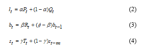where,  denotes the series level at time t,  denotes the slope at time t,  denotes the seasonal component of the series at time t and m denotes the number of seasons in a year; the values  and  vary according to which of the cells the method belongs regarding the combination of the trend and seasonal component,  and  are constants. Additive and multiplicative methods give the same point forecasts but different forecast intervals. To fit an ARIMA and ETS models in R there are many forecasting packages. In our study we have used the forecast v8.3 package managed by Hyndman [33-35].

2.3.  ANN model

In the literature of forecasting it is widely used the fact that ANNs are flexible computing frameworks for modeling a range of nonlinear problems [19]. Although there are some heuristic rules for the selection of the activation function it is not clear whether different activation functions have major effects on the performance of the networks. The single hidden layer feed forward network is widely used for time series modeling and forecasting. The model is characterized by a network of three layers of simple processing units connected by acyclic links. The relationship between the output  and the inputs  has the following mathematical representation:

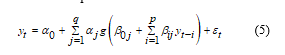where, and   are the model parameters often called the connection weights; p is the number of input nodes and q is the number of hidden nodes. The logistic function is often used as the hidden layer transfer function, f(x)=(1+exp(-x))-1.

Hence, the ANN model of (5) in fact performs a nonlinear functional mapping from the past observations  to the future value , i.e.,

where, w is a vector of all parameters and f is a function determined by the network structure and connection weights.

Both ANN and ARIMA models usually require a large sample in order to achieve a successful forecasting model. It is always advisable to undertake a subjective analysis of the data when choosing among the proposed forecasting models.

2.4. Linear Least Squares Regression  model

Linear least squares regression (LSSVM) is a process which approximates linearly a set of data points ,where x is the input vector, y is the expected output  and n is the number of data. Fundamentally, SVR is linear regression in the feature space. The goal of SVR is to find a function f (x) that deviates not more than e from the targets y for all the training data, and at the same time, is as flat as possible. LSSVM  have been developed to find the optimally of non-linear regression function .

The optimization problem of LSSVM for regression function is given:

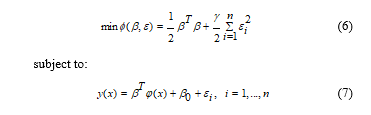LSSVM use a  fitting function is , where are the solution of the linear system and is a Kernel function. The most popular Kernel function is Radial Basis Function [36].{\displaystyle K(x,x_{i})=\exp \left({-\left\|{x-x_{i}}\right\|^{2}/\sigma ^{2}}\right),} {\displaystyle d}

3. Baseline scenario forecasting

Time series models and neural network models are widely used in modeling of time series for prediction purposes. Many studies have shown their performance as separate forecasting models and combined with each other. Interesting results on different nature of time series are presented by Wang L. et al. [29]; Tseng et al [37]; Sheta et al. [38]; Barba et al. [39]. In the field of energy forecasting the studies are focused on choosing one of the models among some of them as has been discussed by many authors [8-9, 11-18, 40-43].

Zhang in his work [20] propose a combination of ARIMA and ANN model with the aim to increase the accuracy of the forecasting dealing both with linear and nonlinear patterns. He present a methodology which first fits an ARIMA model to the real data and then an ANN model to the residuals of the first model dealing this way the nonlinear pattern of the time series. In his study, he show that this methodology increases the accuracy of the forecast on time series data. In their work Khashei and Bijari [44] proposed a hybrid model which first used the ARIMA model to fit the real-time series and then the ANN model to obtain the final forecast. The forecast model seems to have a better performance on the same data set used before by Zhang [20]. Latter, Wang L. et al [29] have presented improvements of Zhang methodology. In 2017, Khairalla et al. [45] proposed a hybrid methodology, using additive multilinear regression methods on forecasting techniques taken as independent variables. They came out with the recommendation that using this hybrid scheme will improve the accuracy of the forecast, especially in the exchange rate time series.

The main strength of SARIMA and ETS is the capability of dealing with linear and seasonal patterns, and combined with the ANN capability of dealing with nonlinear pattern of a time series they are a good combination to offer a potential forecast model for the precipitation and water inflow time series which may be used later to predict the electricity production of the country.

3.1.  Hybrid Methodology Forecast

In the first approach of our work, we propose a hybrid methodology of forecasting models using multiple linear regression method. More precisely, we have used the Least Square Support Vector Machines (LSSVM) [46,47] to the forecasting models (SARIMA, ETS, ANN) with the main goal to assign to each of the models the appropriate weight in final forecast.

Our first approach follows this steps:

Step 1. Fit a forecast model (SARIMA, ETS, and ANN) to the observed data.

Let denote the observation at time t, which will serve as the dependent variable in multiple linear regression model and as independent variables we will use the estimated values obtained from each forecasting model independently. So,  in our case is the estimated time series obtained from a SARIMA model,  is the estimated time series obtained from an ETS model and is the estimated time series obtained from an ANN model.

Step 2. Use the fitted values from the models in step 1 as independent variables to the multiple linear regression model and estimate the weights for each model based on LSSVM (Least Square Support Vector Machines).

Then, the estimated values from the additive multiple linear regression model will be:

      Step 3. Use the multiple linear regression model fitted in Step 2 to obtain the final forecast. Use as input values the forecasted values from each single model (SARIMA, ETS, ANN).

So, after evaluating the coefficients of the model through the LSSVM procedure [46] we obtain the equation which will serve as the final forecasting model of our time series. The forecasted time series from each technique (denoted by , where Model={SARIMA, ETS, ANN} and F stands for Forecast for a given period) serve as input variables in the multilinear regression model:

This procedure will be followed for the time series of precipitations and water inflow in Fierza HPP. At this step we have considered two hybrid models (Hybrid 1 and Hybrid 2) with two and three forecasting models respectively.

3.2.  Improved Hybrid Methodology Forecast

In our second approach we have used the fitted values from the “best” hybrid model (Hybrid 1 or Hybrid 2) obtained in the first approach as “real” observations and we have fitted a SARIMA and ETS model. Then, after the evaluation of the two models (SARIMA, ETS) we obtain the final forecast for the next period.

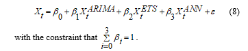
3.3.  Automatic Hybrid Forecast

To compare the forecasting models we have chosen in our third approach an automatic forecasting time series package in R (forecast and forecastHybrid v8.3) managed by Rob J. Hyndman (2018). Forecasts generated from auto.arima(), ets(), thetam(), nnetar(), stlm(), and tbats() can be combined with equal weights, weights based on in-sample errors, or CV weights. The forecastHybrid package includes the ARIMA, ETS and ANN model along with other forecasting techniques. The results are obtained by optimizing the prediction features of the model based on minimizing error. The automatic methodology was applied to the water inflow and precipitation time series and a list of 12 models (single and combined) is obtained.

3.4.    Model Performance measures

In both cases (non-automatic procedure and the automatic procedure) the accuracy of the model is evaluated based on some performance measures: the Mean Error (ME), Mean Absolute Error (MAE), Mean Absolute Percentage Error (MAPE), symmetric MAPE (sMAPE) and Root Mean Square Error (RMSE). The evaluation of the model performance is made based on the lower value of these accuracy measures [48,49]. The selection of the “best” model between all proposed was affected also on subjective indicators observed in the behavior of the time series such as seasonality and production requirements from OSHEE.

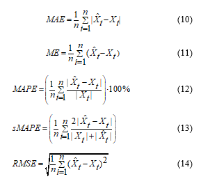where,  denote the observation at time t and  denote the estimated time series .

4. Empirical results and discussion

Since Albania is part of the subtropical belt and included in the Mediterranean climate zone (with short winters and hot-dry summers) the production of electrical energy is mainly based in the level of precipitations (millimeters) and water inflow (m3/sec). According to the Kesh – Gen procedure the year is divided into four energetic periods, which are October-February, March, April-May, June-September. Fierza is the oldest and most important hydropower plant built on the river Drin and thus it has a stronger impact on energy production compared to other HPPs in the country. Also, it has the highest height (or otherwise Hash) which directly determines the output power.

The data are collected every day from January 2011 to February 2018. Considering the fact that the necessity for energy production is long-term we have considered monthly data of precipitations and water inflow. Figure 1 shows the behavior of these time series. Being a country with a Mediterranean climate, it is not a surprise that the water inflow in the HPP is affected by the melting of the snow in mountains but we should not forget that the main impact on water inflow   are precipitations.

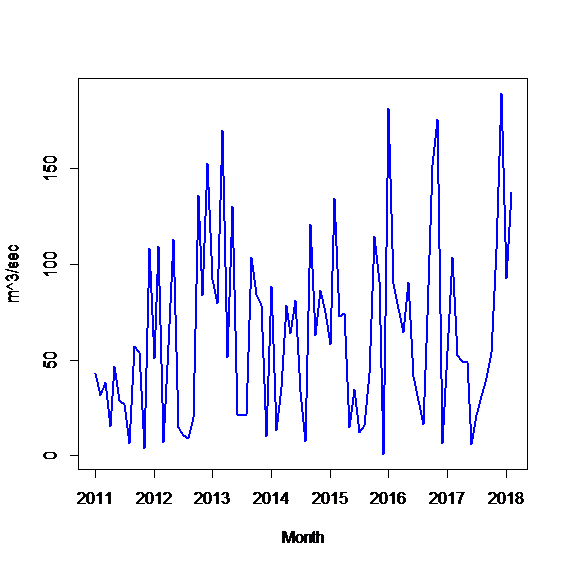Figure 1.a Precipitations (Millimeters) Time series for Fierza HPP(January 2011- February 2018)

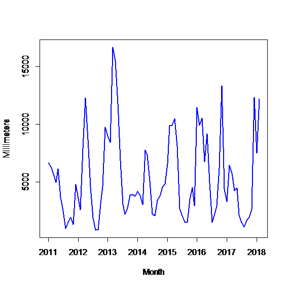Figure 1.b Water inflow (m^3/sec). Time series for Fierza HPP(January 2011- February 2018)

A preliminary pre-processing of the time series of precipitation and water inflow in Fierza show that the trend is not a critical component of the time series. We observe monthly seasonality as well as a climacteric season which plays an important role in the model selection procedure of the forecasting techniques. In figure 1 the trend is “hidden” in the whole time series but if we observe carefully it is present within the season of the time series. Figure 2 shows the presence of trend and seasonality in each time series: precipitation and water inflow for Fierza HPP.

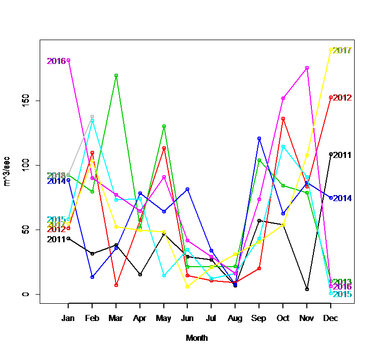Figure 2.a Precipitation (Millimeters), Seasonal plot for Fierza HPP(January 2011- February 2018)

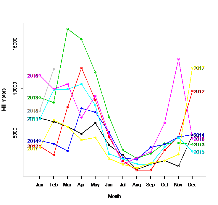Figure 2.b Water inflow (m^3/sec). Seasonal plot for Fierza HPP(January 2011- February 2018)

The seasonal plot of water inflow is more stable compared to that of the precipitation which seems to be mostly affected by the climacteric changes.

4.1.  Results for Hybrid Forecast

Using the forecast package offered in R we have fitted separately the SARIMA, ETS and ANN model for the precipitation and water inflow time series. The corresponding models and parameters are presented in Table 1.

Table 1. The parameters of the SARIMA, ETS and ANN model for the precipitation and water inflow time series

	Precipitation	Water in flow
SARIMA	ARIMA(0,0,0)(1,0,0)[12]	ARIMA(1,0,0)(1,0,0)[12]
Coefficients	sar1=0.1685	ar1=0.6177, sar1=  0.2266
ETS	(M,Ad,M)	(M,N,M)
	alpha=1e-04                           beta=1e-04                       gamma=1e-04               phi=0.9443	alpha=0.1966                                                 gamma = 1e-04
ANN	NNAR(1,1,2)[12]	NNAR(1,1,2)[12]

For the ANN model in both time series there were an average of 20 networks, each of which is a 2-2-1 network with 9 weights. We have tested two multiple linear regression models corresponding with two and three parameters. Based on our non-automatic hybrid model of combining the forecasting models (ARIMA, ETS, ANN) in one multiple linear regression model we have obtained the following results:

Hybrid Model 1: (with two models)

Hybrid Model 2: (with three models)

The computed accuracy measures for each hybrid model are given in Table 2. Analyzing these values we observe that the Hybrid model 2 has a lower value of the errors and s.d. of the errors compared to other models. This is a good sign which shows the importance of each technique on the prediction of precipitation and water inflow time series.

Table 2. Comparison of fitted models for precipitation and water inflow time series in Fierza HPP

Model	Precipitation in Fierza HPP
	RMSE	MAPE	SMAPE	SD
ARIMA	46.722	2.513	0.396	46.996
ANN	40.292	1.992	0.359	40.529
ETS	41.342	2.392	0.299	41.585
Hybrid 1	38.505	2.07	0.322	38.73
Hybrid 2	37.379	1.813	0.269	37.599
Model	Water Inflow in Fierza HPP
	RMSE	MAPE	SMAPE	SD
ARIMA	2860.68	0.545	0.246	2877.46
ANN	2439.6	0.46	0.203	2453.9
ETS	3551.65	0.455	0.194	3572.48
Hybrid 1	2393.31	0.44	0.193	2407.35
Hybrid 2	2376.64	0.43	0.19	2390.58

We have used MAPE as a popular measure for forecast accuracy and the calculated value for Precipitation Hybrid 2 model is 1.813% which is the lower value between the proposed models; and for Water in-flow Hybrid 2 model has again the lower value compared to other models, 0.43% error.

A view of the real-time series, fitted and forecasted values from the hybrid models (Hybrid 1, Hybrid 2) for precipitation and water inflow time series data in Fierza are shown in Figure 3.a and Figure 3.b respectively. From the graphical representations, we may observe that the multi-linear regression model (Hybrid 2) offers a good approximation to the real-time series data compared to Hybrid 1 model.

The water inflow time series for Fierza HPP show stationary patterns and with a clear seasonal behavior which makes it easier to model the time series and obtain accurate predictions.

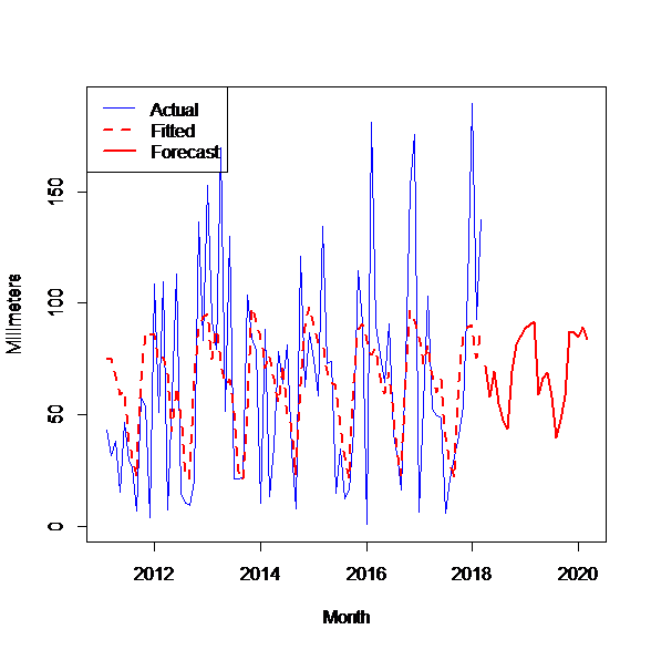Figure 3.a Hybrid model 1, time series of precipitation real, fitted and forecast

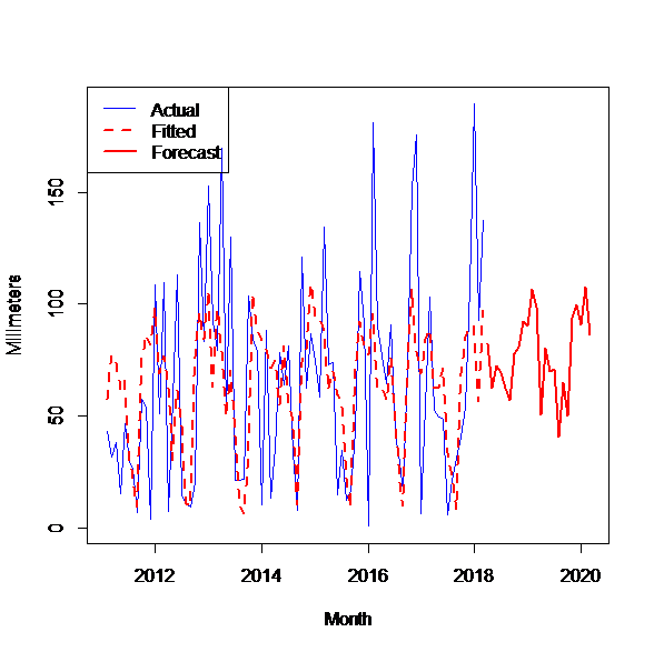Figure 3.b Hybrid model 2. Time series of precipitation real, fitted and forecast

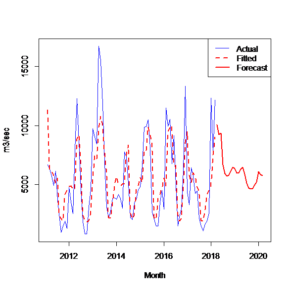Figure 4.a  Hybrid model 1. Time series of water inflow real, fitted and forecast

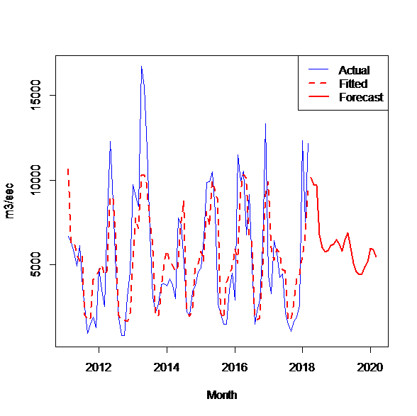Figure 4.b Hybrid model 2. Time series of water inflow real, fitted and forecast

4.2.  Results for Improved Hybrid 2 Forecast

A second approach was considered in order to achieve better predictions on the water inflow times series.  Goodness of fit test for the first approach show that Hybrid 2 model performed better than the Hybrid 1 model. So, in the second approach we use the fitted values from Hybrid 2 model and build a SARIMA model to the fitted values. The results show that a seasonal model with seasonality 12 gives the lower value of the accuracy measures (the characteristics of the fitted model are: ARIMA(0,0,2)(0,1,1)[12], Coefficients: ma1=0.7579, ma2=0.3682, sma1=-0.7012; MAPE=23%). An ETS model was also fitted to the Hybrid 2 values and the best model among the proposed was ETS(M,N,M); Smoothing parameters: alpha = 0.0277, gamma = 1e-04; MAPE=25%.

From the values of the accuracy measures and graphic tests among Hybrid 2 model and the improved Hybrid 2 model, it is noted that the improved model has the best qualities to be used as a predictive model.

For the precipitation time series the SARIMA and ETS model built on the Hybrid 2 fitted values were: SARIMA with seasonality 12 and characteristics SARIMA(0,0,0)(2,1,0)[12], Coefficients: sar1=-0.5886, sar2=-0.3055; MAPE=16.8% .

The ETS(A,N,A) model has the characteristics: Smoothing parameters: alpha = 1e-04, gamma = 1e-04; MAPE=15.9%).

4.3.  Results for Results for Automatic Hybrid Forecast

Using the forecastHybrid v8.3 package in R [34,35] we have obtained the following results among the possible combinations of forecasting models offered by this package. We may notice from the empirical results of accuracy measures (shown in Table 3) that the hybrid model of ANN and STLM (Seasonal and Trend decomposition using Loess) perform better than other models [50]. It has the lower value of RMSE and MAE as well. The ANN model detects the nonlinear behavior of the time series and is therefore important to the model, as well as the seasonal behavior of the model which is detected by STLM. In both time series (precipitation and water inflow in Fierza HPP) the combination of ANN and STLM gives the lower value of accuracy measures.

Table 3. Comparison of models computed from automatic package in R for precipitation and water inflow time series in Fierza HPP

Model	Precipitation in Fierza HPP			Water Inflow in Fierza HPP
	ME	RMSE	MAE	ME	RMSE	MAE
ARIMA	-0.19	49.705	39.58	-170.85	3093.26	2268.99
ETS	-3.98	43.496	32.12	-143.48	3318.93	2084.24
ANN	0.007	41.306	32.67	-0.466	2459.17	1857.74
ARIMA-ANN	-1.61	43.019	34.09	-155.39	2506.95	1839.74
ARIMA-TBATS	6.243	47.632	36.01	61.031	2888.54	1984.21
ANN-STLM	-2.07	38.59	29.43	1.683	2291.94	1626.79
ARIMA-ANN-STLM-TBATS	0.145	40.149	30.9	-15.618	2387.21	1643.96
ANN-TBATS	3.927	40.306	31.23	124.465	2322.08	1644.9
ARIMA-STLM	0.072	43.978	33.57	-122.38	2810.57	1960.62
ARIMA-ANN-STLM	-2.46	40.458	31.42	-103.83	2385.47	1689.96
ARIMA-ANN-TBATS	1.581	41.886	32.68	-19.784	2404.52	1711.96
ANN-STLM-TBATS	1.248	39.038	29.51	82.482	2325.47	1593.13

The closest values of errors after the combined ANN-STLM model are those of the hybrid model ANN-STLM-TBATS which is very close to the Hybrid 2 model proposed at the beginning. Since the differences in value are sufficiently small they can be considered irrelevant, and therefore the two models can serve to provide forecasts in the future.

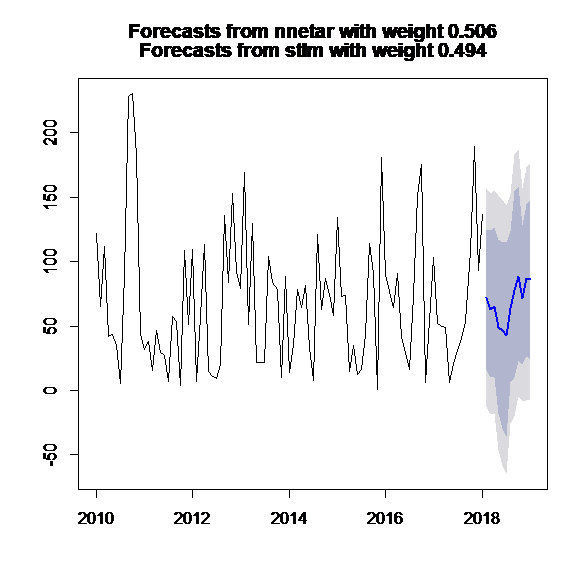Figure 5.a  Precipitation, fitted and forecast from automatic hybrid model in R

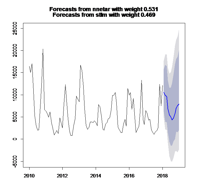Figure 5.b Water inflow real, fitted and forecast from automatic hybrid model in R

Figure 5 shows for precipitation and water inflow time series the real values, fitted and forecasted values obtained from automatic hybrid model (ANN+STLM) in R. Due to the apparent stationarity and seasonal behavior the water inflow time series has good qualities to be modelled.

Figure 6 shows the water inflow: real observations, improved Hybrid 2 based on SARIMA, improved Hybrid model 2 based on ETS, the automatic (ANN+STLM) forecast from the forecast Hybrid v8.3 package and the Hybrid 2 forecast.

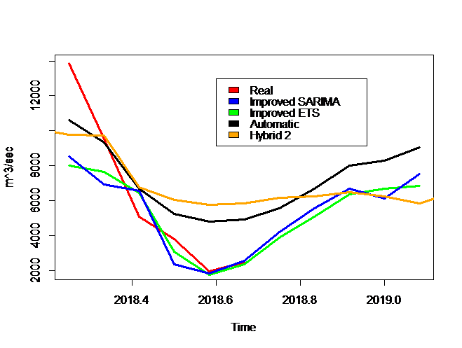Figure 6.   Water inflow: real observations, forecasted values from the improved models (SARIMA and ETS on Hybrid 2 fitted values), the automatic forecast in R and Hybrid 2 forecast (period: April 2018-April 2019)

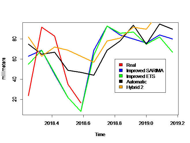Figure 7.   Precipitations: real observations, forecasted values from the improved models (SARIMA and ETS on Hybrid 2 fitted values), automatic forecast in R and the Hybrid 2 forecasted values (period: April 2018-April 2019)

Figure 6 and Figure 7 show a graphical comparison of forecasting results from the Hybrid 2 model, improved Hybrid 2 model and automatics forecast in R. Due to the geographical position and Mediterranean climate of Albania the precipitations are mainly present in two periods: October-February and March. In the case of precipitation time series, it is noticed that the “best” approximation to real observations are obtained from the improved Hybrid 2 model (both SARIMA and ETS show satisfied approximations to real observation compared to other models). And, for the precipitation time series again the improved Hybrid model show a satisfactory approximation to real data. It is known that precipitations are influenced by temperatures and changes in global warming so, the variations between the real values and the forecasted from the improved Hybrid 2 (SARIMA and ETS) are acceptable and within the confidence levels.

5. Conclusions

In this study two main indicators of energy production were analyzed, precipitation and water inflow recorded for every month in the period January 2011- February 2018 for the largest HPP in the country (Fierza HPP) which has the main impact on electricity production. After a detailed analysis of the characteristics of the time series: trend, seasonality, and randomness we have considered hybrid models in order to obtain an accurate prediction for the upcoming months. In this work we present three methodologies: Hybrid models based on LSSVM method; improved Hybrid models with SARIMA and ETS forecasting models and automatics hybrid models proposed by forecastv8.3 package in R. The water inflow time series is the most regular; therefore, it is easier to achieve a qualitative forecasting method compared to the precipitation time series which show irregular patterns and has therefore a lower accuracy level.

The challenge of this work was to show that not all the proposed methodology on forecasting are effective because they depend on the nature of the time series. Especially, for the hydrological time series which are affected from various unstable factors it is necessary to work on many techniques and combinations to achieve the best accuracy forecast model. The improved hybrid model proposed in this study was considerably more effective compared to the models proposed earlier in the literature.

Conflict of Interest

The authors declare no conflict of interest.

1. Bates, J.M.; Granger, C.W.J. The combination of forecasts, Oper. Res. Q. 1969, 20, 451–468.
2. Box, G. E. P.; Jenkins, G. Time Series Analysis: Forecasting and Control, Oakland, CA: Holden-Day, 1976.
3. Chatfeld, C., What is the ‘best’ method of forecasting? J. Appl. Statist. 1988, 15, 19–39.;
4. Makridakis, S.; Anderson, A.; Carbone, R.; Fildes, R.; Hibon, M.; Lewandowski, R.; Newton, J.; Parzen, E.; Winkler, R.; The accuracy of extrapolation (time series) methods: results of a forecasting competition, J. Forecasting, 1982, 1, 111–153.
5. Makridakis, S. Why combining works? International Journal of Forecasting, 1989, 5, 601–603.
6. S.; Chatfeld, C.; Hibon, M.; Lawrence, M.; Millers, T.; Ord ,K.; Simmons, L.F. The M-2 competition: a real-life judgmentally based forecasting study, International Journal of Forecasting, 1993, 9, 5–29. https://en.wikipedia.org/wiki/Makridakis_Competitions
7. Yu, L.; Wang, Sh.; Lai, K. K.; Nakamori, Y. Time series forecasting with multiple candidate models: selecting or combining, Journal of Systems Science and Complexity,2005, Vol. 18 No. 1.
8. Gjika, E.; Ferrja, A.; Efficiency of Time Series Models on Predicting Water Inflow (Case Study, Drin river in Albania), Proceedings of the 3rd Virtual Multidisciplinary Conference, Slovakia, December, 7- 11, 2015, Publisher: EDIS – Publishing Institution of the University of Zilina, http://doi.org/10.18638/quaesti.2015.3.1.225
9. Simoni, A.; Dhamo (Gjika), E. Evolutionary Algorithm PSo and Holt-Winters method applied in hydro Power Plants Optimization. Proceedings of the STATISTICS, PROBABILITY & NUMERICAL ANALYSIS 2015 METHODS AND APPLICATIONS Conference, Albania, December 5-6, 2015. ISSN 2305-882X. https://sites.google.com/a/fshn.edu.al/fshn/home/botim-special
10. Simoni, A.; Dhamo (Gjika), E. Forecasting the maximum power in hydropower plant using PSO, Proceedings of the 6th INTERNATIONAL CONFERENCE Information Systems and Technology Innovations: inducting modern business solutions, Tirana, Albania, June 5-6, 2015. ISBN: 978-9928-05-199-8.
11. Suhartono, S.P.; Prastyo, D.D.; Wijayanti, D.G.P.; Juliyanto, Hybrid model for forecasting time series with trend, seasonal and salendar variation patterns, IOP Publishing, IOP Conf. Series: Journal of Physics: Conf.Series 890,2017, 012160, https://doi.org/10.1088/1742-6596/890/1/012160
12. Ozozen, A.; Kayakutlu, G.; Ketterer, M.; Kayalica, O. A Combined Seasonal ARIMA and ANN Model for Improved Results in Electricity Spot Price Forecasting: Case Study in Turkey, Proceedings of Portland International Conference Management of Engineering and Technology (PICMET),2016, 2681–2690.
13. Wulansari, R.E.; Setiawan, Suhartono, A Comparison of Forecasting Performance of Seasonal ARIMAX and Hybrid Seasonal ARIMAX-ANN of Surabaya’s Currency Circulation Data, International Journal of Management and Applied Science, 2016, Vol.2, Issue-10, ISSN: 2394-7926
14. Wangsoh, N.; Watthayu, W.; Sukawat, D. A Hybrid Climate Model for Rainfall Forecasting based on Combination of Self-Organizing Map and Analog Method, Sains Malaysiana, 2017, 46, 12, 2541–2547,
15. http://dx.doi.org/10.17576/jsm-2017-4612-32
16. Khandelwal, I.; Adhikari, R.; Ghanshyam, V. Time Series Forecasting using Hybrid ARIMA and ANN Models based on DWT Decomposition, Proceedings of International Conference on Intelligent Computing, Communication & Convergence (ICCC-2015), India, 2015, Procedia Computer Science, 48, 173-179, http://doi.org/10.1016/j.procs.2015.04.167
17. Hamzaçebi, C. Primary energy sources planning based on demand forecasting: The case of Turkey, Journal of Energy in Southern Africa, 2016, Vol.27, No.1
18. Szolgayová, E.P.; Danaċová, M.; Komorniková, M.; Szolgay, J. Hybrid Forecasting of Daily River Discharges Considering Autoregressive Heteroscedasticity, Slovak Journal of Civil Engineering, 2017, 25, 2, 39-48, http://doi.org/10.1515/sjce-2017-0011
19. Du, Y.; Cai, Y.; Chen, M.; Xu, W.; Yuan, H.; LI, T. A Novel Divide-and-Conquer Model for CPI Prediction Using ARIMA, Gray Model and BPNN, Proceeding of 2nd International Conference on Information Technology and Quantitative Management (ITQM 2014), Moscow, Russia, 2014, Procedia Computer Science, 31, ISBN: 978-1-63266-899-8.
20. Zhang, G.; Patuwo, B. E.; Hu, M.Y. Forecasting with artificial neural networks: The state of the art, International Journal of Forecasting ,1998, 14, 35–62
21. Zhang, G. P. Time Series Forecasting Using a Hybrid ARIMA and Neural Network Model. Neurocomputing. 2003, 50, 159–175.
22. Qi, M.; Zhang, G.P. Tend Time-Series Modeling and Forecasting with Neutral Networks, IEEE Transactions on Neutral Networks, 2008, 19, 5. http://doi.org/10.1109/TNN.2007.912308
23. Talari, S.; Shafie-khah, M.; Osório, G.J.; Wang, F.; Heidari, A.; Catalão, J.P.S. Price Forecasting of Electricity Markets in the Presence of a High Penetration of Wind Power Generators. Sustainability, 2017, 9, 2065. http://doi.org/doi:10.3390/su9112065
24. Papaioannou, G.P.; Dikaiakos, C.; Dramountanis, A.; Papaioannou, P.G. Analysis and Modeling for Short- to Medium-Term Load Forecasting Using a Hybrid Manifold Learning Principal Component Model and Comparison with Classical Statistical Models (SARIMAX, Exponential Smoothing) and Artificial Intelligence Models (ANN, SVM): The Case of Greek Electricity Market. Energies 2016, 9, 635. doi: 10.3390/en9080635
25. Hasanov, F.J.; Hunt, L.C.; Mikayilov, C.I. Modeling and Forecasting Electricity Demand in Azerbaijan Using Cointegration Techniques. Energies 2016, 9, 1045. doi: 10.3390/en9121045
26. Liang, Y.; Niu, D.; Cao, Y.; Hong, W.-C. Analysis and Modeling for China’s Electricity Demand Forecasting Using a Hybrid Method Based on Multiple Regression and Extreme Learning Machine: A View from Carbon Emission. Energies 2016, 9, 941. doi: 10.3390/en9110941
27. Candelieri, A. Clustering and Support Vector Regression for Water Demand Forecasting and Anomaly Detection. Water 2017, 9, 224. doi: 10.3390/w9030224
28. Ma, X.; Liu, D. Comparative Study of Hybrid Models Based on a Series of Optimization Algorithms and Their Application in Energy System Forecasting. Energies 2016, 9, 640. doi: 10.3390/en9080640].
29. Wang, L.; Zou, H.; Su, J.; Li, L.; Chaudhry, S. An ARIMA ANN hybrid model for time series forecasting, Wiley-Syst. Res. and Behav. Sci., 2013, 30, 3, 244–259.        https://doi.org/10.1002/sres.2179
30. Holt, C.C. Forecasting Seasonals and Trends by Exponentially Weighted Moving Averages. ONR Memorandum, Vol. 52, 1957,Carnegie Institute of Technology, Pittsburgh. Available from the Engineering Library, University of Texas, Austin
31. Hyndman, R. J.; Khandakar, Y. Automatic Time Series Forecasting: The forecast Package for R, Journal of Statistical Software, 2008, 27, 3. http://doi.org/10.18637/jss.v027.i03
32. Hyndman, R. J.; Koehler A. B.; Snyder R.D.; Grose S. A state space framework for automatic forecasting using exponential smoothing methods, International Journal of Forecasting, 2002, 18(3), 439–454.
33. Taylor, J. W. Exponential smoothing with a damped multiplicative trend, International Journal of Forecasting, 2003, 19, 715–725.
34. https://cran.r-project.org/web/packages/forecastHybrid/forecastHybrid.pdf
35. https://robjhyndman.com/hyndsight/forecast83/
36. Cristianini, N.; Shawe-Taylor, J. An Introduction To Support Vector Machines and Other Kernel Based Learning Methods. Cambridge, Cambridge University Press. New York, USA, 2000, ISBN:0-521-78019-5
37. Tseng, K-C.; Kwon O.; Tjung L. Time series and neural network forecast of daily stock prices, Journal of Investment Management and Financial Innovations, 2012, 9 (1). ISSN 1810-4967 (print), 1812-9358 (online)
38. Sheta, A.; Ahmed, E.; Faris, S.H. A Comparison between Regression, Artificial Neural Networks and Support Vector Machines for Predicting Stock Market Index , International Journal of Advanced Research in Artificial Intelligence, 2015, 4 (7) , 55-63. http://doi.org/10.14569/IJARAI.2015.040710
39. Barba, L.; Rodriguez, N.; Montt, C. Smoothing Strategies Combined with ARIMA and Neural Networks to Improve the Forecasting of Traffic Accidents, Hindawi Publishing Corporation, The Scientific World Journal, 2014, Article ID 152375, 12 pages http://dx.doi.org/10.1155/2014/152375
40. Salas, J.D. Analysis and Modeling of Hydrological Time Series. In: Maidment, D.R., Ed., Handbook of Hydrology, McGraw-Hill, New York, 1993, 19.1-19.72.
41. Noakes, D.J.; McLeod, A.I.; Hipel, K.W. Forecasting monthly riverflow time series, International Journal of Forecasting, 1985, 179-190, North Holland
42. Collischonn, W.; Tucci, C.E.M.; Clarke, R.; Chou, S.C.; Guilhon, L.G.; Cataldi, M.; Allasia, D. Medium-range reservoir inflow predictions based on quantitative precipitation forecasts. Journal of Hydrology. 2007, 344. 112-122. http://doi.org/10.1016/j.jhydrol.2007.06.025
43. Sulandari, W.; Subanar S.; Suhartono S.; Utami H.. Forecasting electricity load demand using hybrid exponential smoothing-artificial neural network model, International Journal of Advances in Intelligent Informatics, 2016, 2(3), 131-139, ISSN: 2442-6571, https://doi.org/10.26555/ijain.v2i3.69
44. Khashei, M.; Bijari, M. A novel hybridization of Artificial Neural Networks and ARIMA models for time series forecasting, Appl. Soft Comput., 2011, 11(2), 2664–2675. https://doi.org/10.1016/j.asoc.2010.10.015
45. Khairalla, M.; Xu-Ning; Nashat, T.; AL-Jallad. Hybrid Forecasting Scheme for Financial Time-Series Data using Neural Network and Statistical Methods, International Journal of Advanced Computer Science and Applications (IJACSA), 2017, 8(9). http://dx.doi.org/10.14569/IJACSA.2017.080945
46. Suykens, J.A.K.; Vandewalle, J. Least squares support vector machine classifiers, Neural Processing Letters, 1999, 9 (3), 293-300. https://doi.org/10.1023/A:1018628609742
47. Wang, H.; Hu, D. Comparison Of SVM And LSSVM For Regression. Proceedings of International Conference on Neural Networks and Brain, Beijing, 2005, 1: 279–283
48. Hyndman, R. J.; Koehler, A. B. Another look at measures of forecast accuracy. International Journal of Forecasting, 2006, 22(4), 679-688. https://doi.org/10.1016/j.ijforecast.2006.03.001
49. Hyndman, R. J. Measuring forecast accuracy, 2014, https://pdfs.semanticscholar.org/af71/3d815a7caba8dff7248ecea05a5956b2a487.pdf
50. Cleveland, R. B.; Cleveland, W. S.; McRae, J. E.; Terpenning, I. J. STL: A seasonal-trend decomposition procedure based on loess. Journal of Official Statistics, 1990, 6(1), 3–73.

(Click Here)

(Click Here)