1. Introduction

Many papers have been published about thin region finite element (FE) models [1]-[7]. Besides theoretical studies on the shielding effect and related to interface conditions (ICs), several finite element (FE) subproblem method (SPM) formulations for the thin shell (TS) models have been developed [1]-[7]. This means that instead of meshing the volume thin regions, the TS models can be considered as surfaces with ICs, that neglect errors on the computation of local electromagnetic quantities in the vicinity of geometrical discontinuities, edges and corners, increasing with the thickness [1] – [4].

In this paper, the FE SPM is herein extended for coupling of local fields (magnetic flux density, magnetic field and eddy current) and global quantities (currents, voltages Joule losses) associated with any conducting part of an electric system to correct the inherent errors of the local and global fields near eges and corners comming from the TS models. It is particularly the case with inductors driven by external sources. For such components, either a global current  or a global voltage  can be fixed (Figure 1), in a more general way, both of them must be taken into account when a coupling with circuit equation is performed.

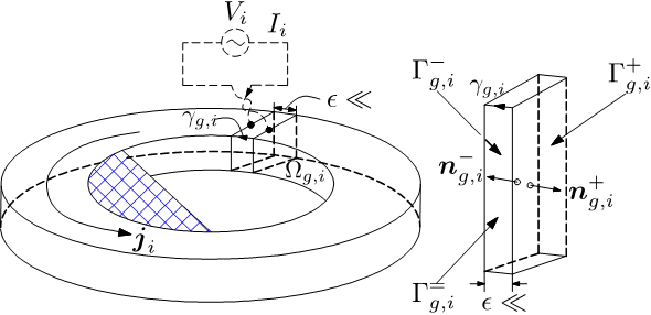Figure 1. Generator W_g,i  with associated global current I_i and voltage V_i.

The FE SPM allows to couple any changes from this problem to others via surface sources (SSs) and volume sources (VSs) and applied via a projection method [1]-[4]. The development of the method is proposed for the magnetic vector potential FE magneto dynamic formulation, paying special attention to the proper discretization of the constraints involved in each subproblem (SP) and to the resulting weak FE formulations. The method is validated on a practical test problem [8].

2. Coupled Magnetic Subproblem

2.1.  Sequence of Subproblems

      At the hearth of the SPM, a full problem is proposed to be divided into sequences of SPs:  A problem involving global current driven stranded or massive inductors alone is first performed on a simplified mesh without any thin regions. The obtained solution considered as SSs for added TS problems via ICs [1] – [7]. The TS solution is then corrected by a correction problem via SSs and VSs, that overcomes the TS assumptions as presented in  Section 1.

2.2.  Canonical magneto dynamic problem

A canonical 3-D magnetodyanmic problem i, to be solved at step i of the SPM, is defined in a domain , with boundary . The eddy current defined in the conducting part and the non-conducting of  are respectively denoted  and , with  . Stranded inductors belong to , whereas massive inductors belong to . The equations and material relations of SPs i are [9] – [11]:

where  is the magnetic field,  is the magnetic flux density,  is the electric field,  is the electric current density,  is the magnetic permeability and ­ is the electric conductivity. Note that (c) is only defined in   , whereas it is reduced to the form (1b) in . Boundary conditions (BCs) are defined on complementary parts  and   , i.e.

where n is the unit normal exterior to . The surface fields   and   in (3a) and (3b) are SSs which comes from previous problems [2] – [6].  For the classical homogeneous BCs, they normally define as zero. However, they define as possible SSs in the thin region between  and  [1] – [7]. This is the case when some field traces in a  are forced to be discontinuous, whereas their  continuity must be recovered via a . The SSs in  are thus to be fixed as the opposite of the trace solution of .

In addition, global conditions on currents or voltages in inductors are considered. A typical inductor is shown in Figure 1 where a source of electromotive force  is defined between two electrodes very close to each other of voltage  and the current  following through surface  , i.e.

where  is a path in  connecting its two electrodes. Surface  is defined as a part of the boundary  of the studied domain in presences symmetry conditions.

    The fields  and  (fixes the global current in inductors) and in (2a) and (2b) are VSs which can be used for expressing changes of materials in each SP [1]-[4]. Indeed, for changes of permeability and conductivity in a region, from  (i = u) to  (i = p) are defined via VSs  and , i.e.

       Each SP is constrained through the so defined SSs and VSs from the parts of the solutions of other SPs.

3. Finite Element Weak Formulation

3.1.  Magnetic Vector Potential Formulation

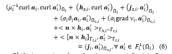
We can define a vector potential   so that  and . A weak formulation of  (iº u, p or k) of the Ampère equation (1a) can be written as [1]-[4].

where  is a curl-conform function space defined in , gauged in , and containing the basis functions for  as well as for the test function  (at the discrete level, this space is defined by edge FEs; the gauge is based on the tree-co-tree technique); (·, ·)W and < ·, · >G respectively denote a volume integral in W and a surface integral on G of the product of their vector field arguments. The surface integral term on  is considered as natural BCs of type (3a), usually zero. The electrical scalar potential  is only defined in the conducting regions . The weak formulation (6) implies, by taking  as a test function, that

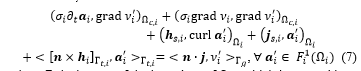where  is the part of the boundary of  which is crossed by a current (  is the union of all the surfaces  resulting from the abstraction of the generators ) (Fig. 1).

3.2.  Current as weak global quantities and circuit relations

   For the weak formulation in (6), the appearing of total current in a conductor is only expressed in a weak sense, e.g. as a natural global constraint, because it arises from Ampère law which is its self-expressed in a weak form. By solving the equation (7), the current  flowing in the part  of an inductor can be obtained with  equal to the source scalar potential . Hence, with , the surface intergral term in (7) written for the inductor  gives

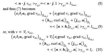Equation (10) is the circuit relation associated with the inductor , i.e. a relation between its voltage  and its current .

3.3.   Inductor alone  – The added TS model  – Volume correction

The weak form of an  with the inductor alone is first solved via the volume integrals in (10) (i º u) where   is the fixed current density in on , i.e.

The added TS problem is defined via the second term in (11) (i º  p). The test function  is divided into continuous and discontinuous parts   and   (with   zero on ) [6]. One thus has

The terms of the right-hand side of (12) are developed from the TS models [6], i.e.

The surface integral term  in (14) is considered as a SS appeared from the weak formulation of  (6), i.e.

At the discrete level, the first term on the right side of (15)  is thus limited to a single layer of FEs on the side  touching , because it occurs only the associated trace . Moreover, the source  obtained from the mesh of  is then projected on the mesh of  via a projection method [1] – [7].

   Once achieved, the  errors on the TS  solution is then corrected by  (i º k) via the volume integrals and in (10). The VSs  and    are given in (4a-b).  In parallel with the VSs in (10), ICs recover the TS discontinuities to remove the TS representation via SSs opposed to previous TS ICs.

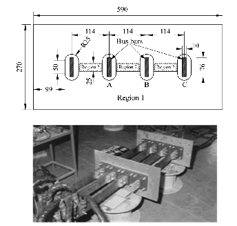Figure 2. The geometry of the cover plate (top) and the experimental set-up (bottom) (all dimensions are in mm).

4. Application example

The illustrate and validate the SPM with global quantities, an actual test problem is a cover plate of a transformer with ratings from 500kVA upto 2000kVA. The geometry of the cover plate is shown in Figure 2 (top) and the experimental set – up developed by the authors in [8] is presented in Figure 2 (bottom).

The three bus bars carry adjustable balanced three – phase currents up to ,   and . The distance between plates is 114mm and the plate dimensions are 270x590x6mm (Figure 2, top). The cover plate is made of two different regions and properties (magnetic and non-magnetic). The conductivities for the regions 1 and 2 are taken as  = 4.07 MS/m and  = 1.15 MS/m respectively and the relative permeabilties for the regions 1 and 2 are taken as  = 300 and  = 1, respectively.

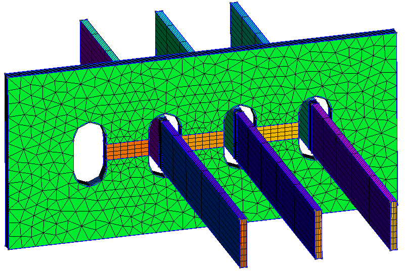Figure 3.  The three – dimensional mesh of the cover plate.

The 3-D – dimensional mesh of the cover plate is shown in Figure 3, with line terminations of the three phases. The non-magnetic material inserted in region 2 (25mm wide) can also be clearly seen in both Figure 2 and Figure 3.

The problem herein is considered three SPs strategy.  The field  computed in a simplified mesh in  (with the bus bars considered as massive inductors) is shown in Figure 4 (top). A TS model  (presenting the distribution of eddy current density  on the surface) is then added (Figure 4, middle). Finally, a  replaces the TS model with volume correction covered by the actual plate and its neighborhood with an adequate refined mesh (Figure 4, bottom). By integrating the value of   (Figure 4, bottom) along the thickness of the cover plate and comparing the result to the TS solution , it is obtained. Thus, the TS inaccuracy on  can locally reach 47% (Fig. 4, middle) (d = 6 mm, f = 50Hz, skindepth  The error on TS  solution through the cover plate hole (Figure 5), and along the cover plate border and near the plate ends (Figure 6) can reach 37,5% and 50%, respectively. The Joule losses and the global currents flowing in the bus bars calculated for the mounting plate (with non-magnetic (region 2) inserted) by the SPM and the experimental method proposed by authors in [8], are given in Table 1. It can be shown that there is a very good agreement.

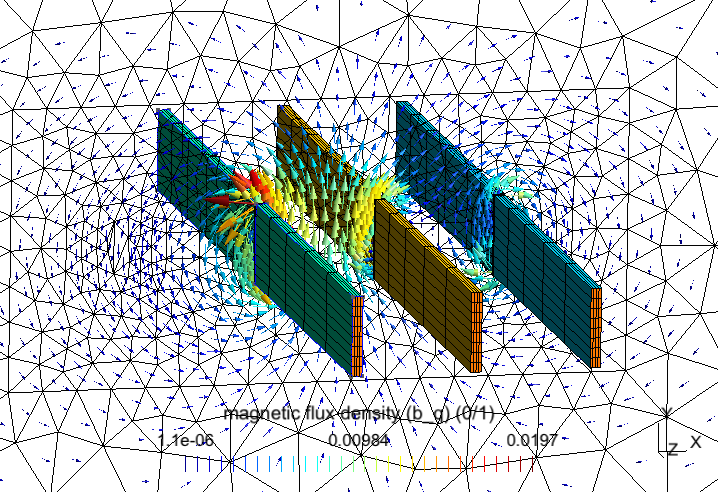
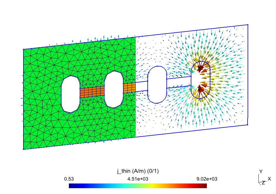
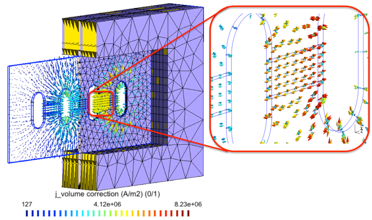Figure 4. Magnetic flux density  (in a cut plane) generated by massive inductors (top), TS eddy current  (middle) and its volume correction  (bottom) (thickness d = 6mm, frequency f = 50Hz).

     This test problem has helped to standardize the type and material of the cover plate for various current in transformers rated between 50kVA upto 2000kVA.

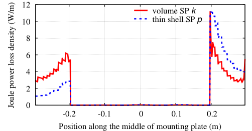Figure 5. Joule power loss density for the TS and VS solution through the plate hole (I_max = 2kA).

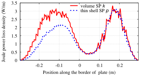Figure 6. Joule power loss density for the TS and VS solution along the plate (I_max = 2kA).

Table 1. Comparison of the computed and measured Joule losses [8] in the cover plate.

Current I (kA)	Frequency f (Hz)	Massive inductors		Measured values (W)
		Thin shell Pthin (W)	Volume Pvol (W)
2000	50	51.8	62.58	65
2250	50	64.8	78.9	74
2500	50	80.8	97.5	95
2800	40	100.5	122.7	119

5. Conclusions

All the steps of the SPM have been extended for coupling of local and global quantities in the magnetic vector potential formulation. The accurately correcting on the local fields and the global quantities are successfully obtained at the edges and corners of the TS FEs mdoels. The method has been performed for coupling SPs in three steps. In addition, it also allows to take advantage solutions from previous  SPs for new problems (with any change of geometrical and physical data) instead of solving again a new complete problem.

1. Vuong Q. Dang, P. Dular R.V. Sabariego, L. Krähenbühl, C. Geuzaine, “Subproblem Approach for Modelding Multiply Connected Thin Regions with an h-Conformal Magnetodynamic Finite Element Formulation”, in EPJ AP., vol. 63, no.1, 2013.
2. Vuong Q. Dang, P. Dular, R.V. Sabariego, L. Krähenbühl, C. Geuzaine, “Subproblem approach for Thin Shell Dual Finite Element Formulations,” IEEE Trans. Magn., vol. 48, no. 2, pp. 407–410, 2012.
3. Dular, Vuong Q. Dang, R. V. Sabariego, L.  Krähenbühl and C. Geuzaine, “Correction of thin shell finite element magnetic models via a subproblem method,” IEEE Trans. Magn., Vol. 47, no. 5, pp. 158 –1161, 2011.
4. Dang Quoc Vuong “A Subproblem Method for Accurate Thin Shell Models between Conducting and Non-Conducting Regions,” The University of Da Nang Journal of Science and Technology, no 12 (109).2016.
5. Tran Thanh Tuyen, Dang Quoc Vuong, Bui Duc Hung and Nguyen The Vinh “Computation of magnetic fields in thin shield magetic models via the Finite Element Method,” The University of Da Nang Journal of Science and Technology, no 7 (104).2016.
6. Dang Quoc Vuong “Modeling of Electromagnetic Systems by Coupling of Subproblems – Application to Thin Shell Finite Element Magnetic Models,” PhD. Thesis (2013/06/21), University of Liege, Belgium, Faculty of Applied Sciences, June 2013.
7. Dang Quoc Vuong, Bui Duc Hung and Khuong Van Hai “Using Dual Formulations for Correction of Thin Shell Magnetic Models by a Finite Element Subproblem Method,” The University of Da Nang Journal of Science and Technology, no 6 (103).2016.
8. V. Kulkarni, J.C. Olivares, R. Escarela-Prerez, V. K. Lakhiani and J. Turowski “Evaluation of Eddy Current Losses in the Cover Plates of Distribution Transformers,” IEE Proc. Sci. Meas. Technol, Vol. 151, No. 5, September 2004.
9. Dang Quoc Vuong “An iterative subproblem method for thin shell finite element magnetic models,” The University of Da Nang Journal of Science and Technology, no 12 (121).2017.
10. Tran Thanh Tuyen and Dang Quoc Vuong, “Using a Magnetic Vector Potential Formulation for Calculting Eddy Currents in Iron Cores of Transformer by A Finite Element Method,” The University of Da Nang Journal of Science and Technology, no 3 (112), 2017 (Part I).
11. Koruglu, P. Sergeant, R.V. Sabarieqo, Vuong. Q. Dang, M. De Wulf  “Influence of contact resistance on shielding efficiency of shielding gutters for high-voltage cables,” IET Electric Power Applications, Vol.5, No.9, (2011), pp. 715-720.

(Click Here)

(Click Here)