1. Introduction

This paper inspired from numerous researchers in science and engineering where there have been discuss the steady-state problems which refer to Fractional Boundary Value problems (FBVPs) since this problem become more attractive in the recent years in many applications such as mathematics, engineering, economy, and other fields [1,2]. Since the rapid growth of computer technology, the numerical techniques are used to solve the large size problem. Following that, there are many researcher have been proposed numerical methods to solve the FBVPs such as Fix et al [3] applied the Least Squares Finite-element methods, Li et al [4] applied the Reproducing Kernel method, Odibat et al [5] applied the Modified Homotopy Perturbation method, and Diethelm et al [6] applied the Extrapolation method. For instance, Sunarto et al [7] started the study on the finite different method to solve the unsteady-state problems using application of the SOR method. In addition, Sunarto et al [8] extended the study with the application of the full-sweep AOR iteration concept to the same problem. Furthermore, this study extend the study to steady-state problems and focus to two-point Fractional BVPs. The problem will be solved numerically and represented as follows [9]:

with the Dirichlet boundary conditions,

where , ,  and  are known functions or constants respectively. Then the derivative term of fractional order is  and the parameter represent fractional order with the range in this study consider as . To get the approximate solution of two-point FBVPs must be discretized to form an approximation equations. Based on the family of FD schemes and Caputo’s fractional derivative operator, the approximation equations use to construct a linear system at each point.

For solving the linear systems which have large and sparse, there are several concept iterative methods from previous researchers have been discussed [10,11]. Other than that, Rahman et al. [12] studied the numerical solution of two-point FBVPs based on the iterative method where SOR method has been used and AGE method in studied Rahman et al. [13]. From the studied, this paper focus to expand the iterative method to the half-sweep scheme. The idea come from Abdullah (1991) who initiated of Half-sweep iteration which is ones of the common utilized use iterative techniques to solve any linear systems. Following that, in this paper proposed 4HSEGSOR iterative method as linear solver to increase the iteration convergence rate so as to solve the two-point FBVPs on the Caputo’s FD approximation equation. To demonstrate the capability of the 4HSEGSOR method, the implementation of the Half-Sweep SOR (HSSOR) iterative method also considered as comparison method in this study and Full-Sweep SOR (FSSOR) iterative methods react as a control method.

After that, the approximation equation will be construct for the problem (1) based on the HS second-order Caputo’s fractional operator via fractional derivative theory. Therefore, let discuss some definitions that can be applied to construct the approximation equation towards problem (1) by using the Caputo’s fractional derivative operator.

Definition 1 [14]. The definition of fractional integral operator for Riemann-Liouville,  of order  given by:

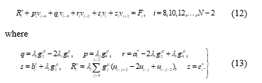
Definition 2 [14]. The definition of Caputo’s fractional derivative operator,  of order  given by:

Where parameter  refer to    and

Definition 3 [15]. The function of Gamma denoted by  is a generalization of factorial function for complex argument with positive real part it is defined as:

To solve the problem (1) as mentioned in early section, we get numerical approximations by using fd scheme via the Caputo’s derivative definition with Dirichlet boundary conditions and fractional derivative operator. In addition to that, the existence and uniqueness of the solution for the problem (1) can be referred and discussed by Diethelm in 2002 in the study Analysis of Fractional Differential Equations [16].

Theorem 4 (existence) [16]. Assume that   with some  and let the function  be continuous. Furthermore, define  Then there exists a function  solving the initial value problem (1).

Theorem 5 (uniqueness) [16]. Assume that     with the . Besides that, let the function  be bounded on  and fulfill a Lipschitz condition the second variable.

Before solving the problem (1), the solution domain of the problem has been confined to the finite domain , with  whereas the parameter  refers to the fractional order derivative. In order to solve the problem (1), let consider the Caputo’s fractional derivative of order  as:

2. Half-sweep Approximation Equation

Before discretizing problem (1), let the solution domain of the problem be partitioned consistently to facilitate in discretizing process. In order to discretize, we consider some positive integers  which is the number of subintervals  and then the length of grid size are defined as.

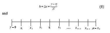Figure 1: The distribution of interior node points over the finite grid network.

From the Figure 1, we develop the consistently grid network of the solution domain where the polar grid of the solution domain will be shown as   and the values of function  at point  are given as . As mentioned in Section 1, the half-sweep concept is imposed to improve the convergence rate. Here the different values of  from the current point to next point between full-sweep and half-sweep is shown in Figures 2 which is Figure 2(a) shows the implementation of the full-sweep iteration which all interior nodes are considered one by one point in which its distance for each point is . However, for half-sweep iteration with its distance  can be seen in Figure 2(b).

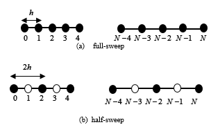Figure 2: The distribution of uniform grid network

After that, to obtain the approximation equation of problem (1), now the equation (5) will be consider to derive based on the formulation of Caputo’s fractional derivative operator which can be gotten by a straightforward quadrature formula as follows.

Then the discrete approximation of equation (6) can be given as

Where can be define by

However, this study don’t use the operator (7) which is shown as the full-sweep Caputo’s fractional derivative since this study focus to the half-sweep concept. Refer to the study of Sonarto et al [17] over the problem, we have propose the half-sweep concept to the Caputo’s fractional derivative operator based on the operator (7) as follows:

As mentioned in Section 1, using the second-order and first-order half-sweep central difference discretization scheme and half-sweep Caputo’s fractional derivative operator (8), the second-order Half-Sweep Caputo’s fd approximation equation for problem (1) given as:

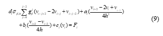
Now, the approximation (9) is known as the half-sweep FD approximation equation it means that the value for each point considers at  refer to the figure 2(b) which show the distribution of grid network. By simplifying (9), the approximation equation can be written as:

Let us define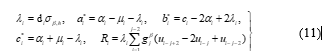

Again, besides the values of , the simplify of approximation equation (9) should be appeared for To simplify the approximation equation, the second-order Half-Sweep Caputo’s FD approximation equation can be expressed as follows:

According to equations (10) and (12), the linear system can be constructed in matrix form to facilitate in solving system of second-order half-sweep Caputo’s approximation equations. As a result, the system of linear equations in the form can be given as:

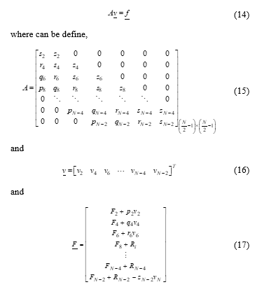
3. Iterative Method

From previous discussion in Section 2 and refer to the linear system equation (14), the formulation of 4HSEGSOR iterative method will be discussed in this section to test the examples than record the numerical results of linear system. Based on the characteristics of the coefficient matrix A, it’s showed the matrix have parse and large-scale. Following to the characteristics, the iterative methods are suitable option to solve the linear system [10]. Besides to improve the consequence rate of iterative method for solving the linear system numerically, there are iterative methods have been proposed from previous researchers such as Jacobi, GS, and SOR methods. However, this study considers the application of 4HSEGSOR method as linear solver as mentioned in early this section.

Particularly, the 4HSEGSOR method is essentially the extension to half-sweep concept for the Four-point Explicit Group SOR (4EGSOR) iterative method which is combination between EG method developed by Evans [18] and SOR method developed by Young [10]. From previous study, Saudi and Sulaiman [19] have been discuss the explicit group to apply into the robot path planning and elucidated the EGSOR iterative method using Nine-Point Laplacian [20] in order to improve the consequence rate of iterative method in the study.

The aim of EGSOR method is to reduce the computational time of the convergence rate by uses small constant size groups strategy based on mesh point and weighted parameter  with its range value given as . However, the main propose of the half-sweep iteration concept in this study is to reduce the computational complexities during iteration process. Following to that, the linear system was divided into several completed small group of four points ( ) start with  . However, for the first three points  can be treated as ungroup case [21]. Since this paper deals with application 4HSEGSOR iterative method for solving the linear system (14), it can be stated as: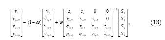

for . To show the illustration, implementation of the 4HSEGSOR iterative method can be shown in Figure 3. Again the first three points, can be stated as ungroup case in which these point can be used to construct the 3-point HSEGSOR method.

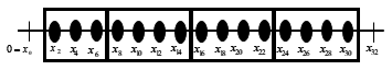Figure 3: Implementation of the half-sweep 4EGSOR iterative method at solution domain m=32.

Based on Figure 3, Algorithm 1 is the implementation of 4HSEGSOR method that be summarized where the optimum values for the parameters, depends on the minimum number of iterations from several executions. The tolerance error set as .

Algorithm 1: 4HSEGSOR iteration

1. Set the value of parameters,
2. Calculate the coefficient matrix, .

• Calculate the vector, .

1. Calculate the value of
2. For calculate an ungroup cases.
3. For calculate again equation (10).
4. Perform the convergence test, If yes, move to step (vi). Otherwise repeat the step (iv).
5. Display approximate solution.

4. Numerical Experiment

This paper demonstrates three examples of numerical experiments for the comparison of two-point FBVPs where the exact solution for each example already given at . Besides that, this paper considers others two different values to analyse the performance of Caputo’s Fractional operator in which   and  refer to Section 1 the range parameter  is . Other than that, three different iterative methods will be implemented such as FSSOR, HSSOR and 4HSEGSOR methods. Beyond that point, considered such as number of iterations (K), computational time measured in second (s) and maximum absolute error (error) as measurement parameters in the numerical experiments need to be recorded while the convergence test considered the tolerance error which is fixed as . The following are three examples of numerical experiments for problem (1).

Example 1

By considering the fractional two point BVP below [22]

With the subject boundary condition as  and , and the exact solution for the problem given  by  when the value of .

Example 2

By considering the fractional two-point BVP below [23]

With the subject boundary condition as  and , and the exact solution for the problem given  by  when the value of .

Example 3

By considering the fractional two-point BVP below [23]

With the subject boundary condition as  and , and the exact solution for the problem given  by  when the value of .

The implementation for the numerical experiments consider the C programing language as a  tools. Following  to  that,  all  the

Table 1. Numerical results on iterative methods for problem 1.

M	Method
		K	Time	Max Error	K	Time	Max Error	K	Time	Max Error
128	FSSOR	751	0.10	2.1230e-02	769	0.13	1.3915e-05	1130	0.12	1.7118e-02
	HSSOR	385	0.02	2.1242e-02	320	0.01	1.3887e-05	385	0.01	1.7188e-02
	HS4EGSOR	132	0.01	2.1242e-02	114	0.01	1.3889e-05	125	0.01	1.7188e-02
256	FSSOR	1483	0.78	2.1228e-02	2051	0.77	1.3924e-05	3547	1.25	1.7081e-02
	HSSOR	765	0.08	2.1230e-02	769	0.09	1.3915e-05	1130	0.10	1.7118e-02
	HS4EGSOR	264	0.02	2.1230e-02	239	0.03	1.3917e-05	285	0.04	1.7118e-02
512	FSSOR	2975	5.62	2.1229e-02	5603	10.68	1.3912e-05	11600	15.90	1.7063e-02
	HSSOR	1522	0.83	2.1228e-02	2130	1.14	1.3922e-05	3525	1.88	1.7082e-02
	HS4EGSOR	512	0.20	2.1228e-02	551	0.19	1.3929e-05	691	0.25	1.7082e-02
1024	FSSOR	6020	33.26	2.1230e-02	15229	58.89	1.3862e-05	11600	199.24	1.7054e-02
	HSSOR	2975	6.25	2.1229e-02	5603	11.70	1.3912e-05	5700	24.29	1.7063e-02
	HS4EGSOR	1005	1.34	2.1229e-02	1309	1.77	1.3933e-05	1883	2.49	1.7063e-02
2048	FSSOR	11785	439.15	2.1230e-02	41071	1281.11	1.3708e-05	123730	1717.04	1.7048e-2
	HSSOR	6020	49.89	2.1230e-02	15229	125.68	1.3862e-05	38179	313.63	1.7054e-02
	HS4EGSOR	1973	10.25	2.1230e-02	3189	16.57	1.3928e-05	5465	28.20	1.7054e-02

Table 2. Numerical results on iterative methods for problem 2.

M	Method
		K	Time	Max Error	K	Time	Max Error	K	Time	Max Error
128	FSSOR	759	0.02	3.2817e-05	769	0.04	8.8991e-04	1110	0.03	3.2013e-02
	HSSOR	382	0.01	3.1865e-02	320	0.01	1.7051e-03	385	0.01	3.2604e-02
	HS4EGSOR	129	0.01	3.1865e-02	112	0.01	1.7051e-03	125	0.01	3.2604e-02
256	FSSOR	1493	0.16	3.3317e-02	2039	0.24	4.6070e-04	3384	0.40	3.1690e-02
	HSSOR	741	0.03	3.2822e-02	769	0.05	8.8708e-04	1110	0.05	3.2010e-02
	HS4EGSOR	259	0.02	3.2822e-02	239	0.02	8.8708e-04	281	0.03	3.2010e-02
512	FSSOR	2826	1.25	3.3570e-02	5478	2.39	2.4094e-04	11330	4.93	3.1521e-02
	HSSOR	1493	0.29	3.3317e-02	2039	0.37	4.6019e-04	3384	0.60	3.1690e-02
	HS4EGSOR	492	0.09	3.3317e-02	541	0.10	4.6019e-04	693	0.15	3.1690e-02
1024	FSSOR	5813	9.88	3.3699e-02	14856	25.44	1.2919e-04	37258	63.29	3.1433e-02
	HSSOR	2826	1.91	3.3570e-02	5478	3.61	2.4085e-04	11330	7.51	3.1521e-02
	HS4EGSOR	1004	0.70	3.3570e-02	1283	0.90	2.4087e-04	1845	1.27	3.1521e-02
2048	FSSOR	11427	77.53	3.3764e-02	40209	271.72	7.2583e-05	121355	820.21	3.1387e-02
	HSSOR	5806	15.14	3.3699e-02	14856	38.43	1.2917e-04	37258	96.54	3.1433e-02
	HS4EGSOR	1975	5.30	3.3699e-02	3121	8.34	1.2924e-04	5349	14.32	3.1433e-02

results of numerical experiments have been recorded based on the iterative methods which are FSSOR, HSSOR and 4HSEGSOR methods in Tables 1, 2, and 3 with three different values of as mentioned in early section. For the grid sizes have used at five different values where the values of m = 128, 256, 512, 1024, and 2048.

5. Discussions of result

Through numerical experiments results from Tables 1, 2, and 3 by imposing the comparison between HSSOR and 4HSEGSOR iterative methods with FSSOR method react as control method as discuss in Section 1 with three different values of parameter , it is conspicuously that number of iterations at Table 1 for HSSOR and 4HSEGSOR  iterative method have declined. The result showed the number of iterations when the parameter set to at size 128 declined from 769 for FSOR to 320 for HSSOR. Again, the number of iterations declined from 320 to 114 for 4HSEGSOR. It’s the same situation for another size the number of iteration has declined. To show more clearly, the percentage of number iterations declined approximately by 82.20% –83.31%, 85.18% – 92.24%, and 83.77% – 95.58% which corresponds to the HSSOR iterative method. For execution time, the result showed 4HSEGSOR method reduce the computational   complexity.   The    execution   time   when   the

Table 3. numerical results on iterative methods for problem 3.

M	Method
		K	Time	Max Error	K	Time	Max Error	K	Time	Max Error
128	FSSOR	712	0.04	2.1230e-02	768	0.07	1.3915e-05	1031	0.06	1.7118e-02
	HSSOR	385	0.01	2.1242e-02	319	0.01	1.3889e-05	378	0.01	1.7188e-02
	HS4EGSOR	126	0.00	2.1242e-02	107	0.00	1.3888e-05	115	0.00	1.7188e-02
256	FSSOR	1397	0.32	2.1228e-02	1988	0.51	1.3926e-05	3272	0.72	1.7081e-02
	HSSOR	712	0.02	2.1230e-02	768	0.06	1.3915e-05	1031	0.04	1.7118e-02
	HS4EGSOR	243	0.02	2.1230e-02	218	0.02	1.3916e-05	247	0.02	1.7118e-02
512	FSSOR	2789	2.44	2.1229e-02	5128	4.34	1.3919e-05	10600	12.24	1.7063e-02
	HSSOR	1397	0.17	2.1228e-02	1988	0.24	1.3926e-05	3272	0.39	1.7082e-02
	HS4EGSOR	473	0.10	2.1228e-02	474	0.10	1.3931e-05	578	0.11	1.7082e-02
1024	FSSOR	5489	19.7	2.1230e-02	13970	54.84	1.3863e-05	34573	136.42	1.7054e-02
	HSSOR	2789	1.24	2.1229e-02	7230	3.18	1.3899e-05	11331	4.95	1.7063e-02
	HS4EGSOR	910	0.66	2.1230e-02	1097	0.79	1.3937e-05	1563	1.19	1.7063e-02
2048	FSSOR	10845	165.55	2.1230e-02	37307	598.82	1.3708e-05	111085	1531.67	1.7048e-02
	HSSOR	5489	9.40	2.1230e-02	13970	23.85	1.3863e-05	34573	59.15	1.7054e-02
	HS4EGSOR	1892	5.28	2.1230e-02	2643	7.28	1.3931e-05	4729	13.02	1.7054e-02

parameter set to  a size 128 declined from 0.13 seconds for FSOR to 0.01 seconds for HSSOR. But, the number of iterations remain same from 0.01 seconds to 0.01 for 4HSEGSOR. It’s the same situation for another size the execution time has reduce. To show more clearly, the percentage of execution time reduced about 90.00% – 97.67%, 92.31% – 98.71%, and 91.67% –98.75% corresponds to the HSSOR method. From the elucidating result for Table 1, the effectiveness 4HSEGSOR can be conform better compare to HSSOR.

In fact, Table 2 show that the numerical experiments for number of iterations HSSOR and 4HSEGSOR iterative method have declined. However, the result showed the number of iterations 4HSEGSOR drastically declined compare with HSSOR. It can be show when the parameter set to  the number of iteration declined from 5478 for FSOR to 541 for 4HSEGSOR meanwhile for HSSOR just to 2039 from 5478. It’s the same situation for another size the number of iteration has drastically declined. To show more clearly, the percentage of number iterations declined approximately by 82.73%–83.00%, 85.44–92.24% and 88.74%–95.60% respectively as compared with the HSSOR method. Also for execution time, the result showed 4HSEGSOR method reduce the computational complexity. The execution time at size 2048 declined from 77.53 seconds for FSOR to 15.14 seconds for HSSOR. Again, the execution time declined from 15.14 seconds to 5.30 seconds for 4HSEGSOR. It’s the same situation for another size the execution time has reduce. To show more clearly, the percentage of execution time reduced about 50.00%–93.16%, 75.00%–96.93%, and 66.67%–98.25% respectively than the HSSOR method. From the elucidating result for Table 2, the effectiveness 4HSEGSOR can be conform more better compare to HSSOR.

Lastly, from the numerical results in Table 3 show that the number of iterations for the 4HSEGSOR iterative method have declined. The result showed the number of iterations at size 512 declined from 2789 for FSOR to 1397 for HSSOR. Again, the number of iterations declined from 1937 to 473 for 4HSEGSOR. It’s the same situation for another size the number of iteration has declined. To show more clearly, the percentage of number iterations declined approximately by 82.30%–83.42%, 86.07%–92.92% and 88.85%–95.74% respectively as compared with the HSSOR method. Also, implementations of computational time for the result showed 4HSEGSOR method reduce the computational complexity. The execution time at size 512 declined from 2.44 seconds for FSOR to 0.17 seconds for HSSOR. Again, the number of iterations declined from 0.17 seconds to 0.10 for 4HSEGSOR. It’s the same situation for another size the execution time has reduce. To show more clearly, the percentage of execution time reduced about 93.75% – 100.00%, 96.08%–100.00% and 97.22%–100.00% respectively than the HSSOR method.

6. Conclusion

For the conclusion, this study success the numerical experiments of the application 4HSEGSOR iteration to solve the linear system generated by the steady-state problems which is two-point FBVPs.  The family FD scheme and Caputo’s fractional derivative operator was applied to construct the linear system. From the linear system, the iterative methods success to applied to get the approximation solution. From the numerical results recorded in Tables 1, 2, and 3 by imposing the comparison between HSSOR and HS4EGSOR iterative methods with FSSOR method react as control method, clearly the results promising two improvements in the number of iterations (K) and execution time (s). According to the numerical results are recorded, it can be showed that the HS4EGSOR method is superior and it has required a much lesser number of iterations and computational time to solve the problems.

Acknowledgment

The authors acknowledge the research grant scheme (GUG0227-1/2018) from Universiti Malaysia Sabah, Malaysia for the completion of this article.

1.  C. Kou, and X. Zhang, “Solutions of the fractional differential equations with constant coefficients.” IEEE. Eighth ACIS International Conference on Vol. 3, pp. 1056-1059, 2007.
2.  D. Matignon, “Stability results for fractional differential equations with applications to control processing.” In Comp eng in systems appl., Vol. 2, pp. 963-968, 1996.
3.  G. J. Fix, and J. P. Roof, “Least squares finite-element solution of a fractional order two-point boundary value problem.” Computers & Mathematics with Applications., 48(7-8), 1017-1033, 2004.
4.  X. Li, H. Li, and B. Wu, “A new numerical method for variable order fractional functional differential equations.” Applied Mathematics Letters., 68, 80-86, 2017.
5.  Z. Odibat, and S. Momani, “Modified homotopy perturbation method: application to quadratic Riccati differential equation of fractional order.” Chaos, Solitons & Fractals., 36(1), 167-174, 2008.
6.  K. Diethelm, & G. Walz, “Numerical solution of fractional order differential equations by extrapolation.” Numerical Algorithms., 16(3-4), 231-253, 1997.
7.  A. Sunarto, J. Sulaiman, and A.Saudi, “Application of The Full-Sweep AOR Iteration Concept for Space-Fractional Diffusion Equation.” IOP Publishing, In Journal of Physics., 710(1), 012019, 2016.
8.  A. Sunarto, J. Sulaiman, and A.Saudi, “SOR method for implicit finite difference solution of time-fractional diffusion equation.” In Proceedings of the 11th Seminar on Science and Technology., pp. 132-139, 2013.
9.  S. Alkan, K. Yildirim, and A. Secer, “An efficient algorithm for solving fractional differential equations with boundary conditions.” Open Physics., 14(1), 6-14, 2016.
10.  Young, D.M., 1971. Iterative solution of large Linear Systems, Academic Press, London, England, Pages:570.
11.  W. Hackbusch, Iterative Solution of Large Sparse Systems of Equations, Springer-Verlag, New York, 1995.
12.  R. Rahman, N. A. M. Ali, J. Sulaiman, and F. A. Muhiddin, “Caputo’s finite difference solution of fractional two-point boundary value problems using SOR iteration.” In American Institute of Physics Conference Series, 2013(2), 2018.
13.  R. Rahman, N. A. M. Ali, J. Sulaiman, and F. A. Muhiddin, “Caputo’s Finite Difference Solution of Fractional Two-Point BVPs Using AGE Iteration.” In Journal of Physics: Conference Series, IOP Publishing, vol. 1123, no. 1, p. 012044. 2018.
14.  I. Podlubny, “Fractional differential equations: an introduction to fractional derivatives, fractional differential equations, to methods of their solution and some of their applications” Academic press, New York, USA., Pages 340, 1999b.
15.  B. R. Sontakke, and A. S. Shaikh, “Properties of Caputo operator and its applications to linear fractional differential equations.” International Journal of Engineering Research and Applications 5, 5(22-29), 2015.
16.  Diethelm, K., & Ford, N. J. Analysis of fractional differential equations. Journal of Mathematical Analysis and Applications, 265(2), 229-248, 2002.
17.  A. Sunarto, J. Sulaiman, and A. Saudi, “August. Solving the time fractional diffusion equations by the Half-Sweep SOR iterative method.” IEEE. In Advanced Informatics: Concept, Theory and Application (ICAICTA), International Conference of pp. 272-277, 2014.
18.  D. J. Evans, “Group explicit iterative methods for solving large linear systems.” International Journal of Computer Mathematics., 17(1), 81-108, 1985.
19.  A. Saudi, and J. Sulaiman, “Block Iterative Method for Robot Path Planning.” In The 2nd Seminar on Engineering and Information Technology (SEIT2009), Kota Kinabalu, Malaysia. 2009.
20.  A. Saudi, and J. Sulaiman, “Robot path planning via EGSOR iterative method using Nine-Point Laplacian.” In 2012 Third International Conference on Intelligent Systems Modelling and Simulation, pp. 61-66. IEEE, 2012.
21.  D. J. Evans, and A. R. Abdullah, “A new explicit method for the diffusion-convention equation.” Computers & mathematics with applications., 11(1-3), 145-154, 1985.
22.  A. El-Ajou, O. A. Arqub, and S. Momani, “Solving fractional two-point boundary value problems using continuous analytic method.” Ain Shams Engineering Journal., 4(3), 539-547, 2013.
23.  A. Pedas, and E. Tamme, “Piecewise polynomial collocation for linear boundary value problems of fractional differential equations.” Journal of Computational and Applied Mathematics., 236(13), 3349-3359, 2012.
24.  H. Azizi, “Chebyshev Finite Difference Method for Fractional Boundary Value Problems.” Journal of Mathematical Extension., 9, 57-71, 2015.

(Click Here)

(Click Here)