1. Introduction

In this era 3D supporting hardware’s are increasing, but the demand of content in 3D and its availability does not go hand in hand. Still 3D contents are surpassed by the 2D contents. So there is a requirement of 3D data and obvious many researchers are already working on this to close this gap in the future. One solution of direct taking 3D using multi-view method is available but it is costly and already there is large amount of 2D data is available; it will be costly to create newly 3D contents. To work on this problem, there should be the technique which convert large amount of 2D available data into 3D. The converted data should have comfortable visual quality and should not time consuming.

The available 2D data is a monocular data, which is taken from using only single view. The main problem in conversion of 2 dimension to 3 dimension  using single image is that it lacks information required for reconstruction in 3D data. As discussed earlier in 2 dimension to 3 dimension  conversion two approaches are available i.e. automatic and semi-automatic. Semiautomatic method gives good results but this method is time consuming and costly. Real time implementation of automatic method is preferable as semi-automatic method requires human intervention and is also known as a most trustable tool in extracting the depth from a particular scene. Disparity-pixels extracting algorithm and the camera quality determines the accuracy of the results.

  2D image depth estimation is usually done in steps. A monochromatic-picture is oulined by depth where a distant separation from a camera is demonstrated by a low intensity and neaby separation is shown by a high power. i.e. it deals with luminance intensity [1]. Thus depth map, as afunction of the image co-ordinates,   presents the depth in corresspondence to the camera position of a point in the visualscene. Estimating depth from a single picture or video quite exciting. As depth is an important cue of a scene which is lost in image acquisition. Because of this reason and several application needs this information, hence various methods are proposed to extract depth.

Depth Image Based Rendering (DIBR) needs a flow of mono-scopic images and a subsequent flow of depth map images that gives details of per pixel depth. Knowing the depth of each point in an input picture, rendering of any close-by perspective into a sample picture can be done by anticipating the pixels of the first picture to their appropriate 3-D areas and re-anticipating them onto the world-picture-plane. In this manner, DIBR grants the formation of novel pictures, utilizing data from the depth maps, as though they were caught with a camera from various perspectives. A favorable position of the DIBR approach is the higher capability with which coding of the depth maps can be done, than two scenes of common pictures, consequently lessening the transfer speed required for transmission. Rendering an image /video has been well realized and there are also very many algorithms available for producing quality and standard images.

In the left image the closer objects to the camera are located in the right while in the right image they are located in the left. The objects farther away from the camera appears in the same place in both the images. The object displacement in the two images is the disparity. The higher depth is indicated by a smaller disparity and a lower depth by a higher disparity. This is why pixel matching between the two images is essential. Output classification into dense and sparse is done on the stereo correspondence algorithms. An optimum mix of speed and accuracy is obtained by applying method of segments & edges.

Real time applications like robotics require dense output. Since our focus was oriented towards algorithms for real time application, the focus was on ‘dense stereo correspondense’. According to [2] dense matching algorithms are divided as  local and global matching. The local one is either area based or feature based. Since the disparity is determined chiefly by the intensity values of a particular window, area-based local method applies variable windows. The window size, depending on the output can be changed such that a dense output is obtained to suit most of the real time applications. The feature extraction on which the feature based methods rely on provides a sparse output. However, they are quite fast.  The accurate global methods, also called the energy based methods are rather very slow and computanionally expensive.

The object/features mapped in both right and left images is assumed to have the same intensity and the algorithms would be implemented. The illumination effects on the objects, with different view points of the cameras, may at times create a diffrence in the intensity values and invalidate these assumptions. Although the two cameras under consideration are completely tuned and both the images are simltaneously captured, stereo vision normally fails in non-ideal lighting. The reason is that the orientation or the pose of the cameras with respect to the light source may result in the variation of the light intensity of the captured images from the respective view points.

Pixel matching is then the whole idea. For this matching the pixels in the left images are to be looked for in the right images. The search becomes difficult if by chance the variations are both in the x and the Y co-ordinates, since the images are captured by to cameras from two different view points.. Image rectification, nothing but the process of horizontally aligning the epipolar lines of the two cameras is deployed to avoid this. Unidirectional alignment is done by means of linear transformations like rotate, skew and translate.

Authors have proposed an automatic 2D to 3D conversion algorithm rooted on multiple depth indications. Three distintive methods were considered for depth generation and consequently 2-D scene one depth generation method was carriedout [3]. The limitation of this method is latency. A few researchers have presented automatic pathway  of learning the 3-D scene structure. In this pathway,  an easier algorithm is recommended that learns the scene depth from a huge store of image + depth pairs. The produced anaglyph images provides a decent  3-D perception. However, they are notabsolutely devoid of distortions.

As image or video is having its attributes at a pixel level that are learned by a point transformation, it is applied to a monocular image.. The limitation of this system is cannot apply same transformation to images with potentially different global 3D scene structure.The same authors have also presented method to automatically convert a monoscopic video into stereo for 3D visualization. They are taking plausible automatically extracted depth maps at every frame and presented a framework using temporal information for improved and time-coherent depth when multiple frames are available. They have mixed indoor and outdoor images; hence indoor images work poor for outdoor images and vice-versa. This system is complex.

Guttmann proposed semi-automatic user defined strokes corresponding to a rough estimate of the depth values are defined for the image of interest in the scene[4]. This particular system finds  the depth values for the rest of the image, and produces  a depth map in order to create stereoscopic 3D image pairs. This can be further extended to automatic method.

This paper proposes the use of image rectification after the calibration of the camera.

The remainder of this brief is arranged as follows. Section II provides the process block diagram and its explanation. Section III presents the simulation results, Section IV subjective analysis and Section V draws the conclusion.

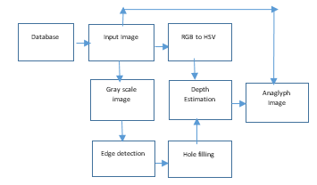Figure 1.Block diagram of process

2. Process Block Diagram

2.1.  Process flow

In 2D-to-3D conversion, input is a RGB monocular color image. Bit depth gives number of bits per pixel and here bit depth should be 24 as the input expected is a RGB image. As an input one can give image of  file formats JPEG, BMP and PNG. Figure 1 is the block diagram of the whole process.

The input image is taken from database. Four datasets are used i.e. Make3D dataset [5], NYU dataset [6], Middlebury dataset [7] and our own dataset. Make3D dataset  is of outdoor images. It consists of 534 images, each is having 1704X272 dimensions.

The NYU-depth v2 dataset is involved video grouping from assortment scenes taken indoor captured by both RGB and Depth cameras of Microsoft Kinect. This dataset  consists of indoor scenes like basements, bedrooms, bathrooms, bookstores, cafe, classroom, dining rooms, kitchens, living rooms, offices etc. Middlebury dataset  is one of the well-known dataset, which comprised of stereo images of various scenes along with its ground truth. We also have created indoor dataset of 22 images each image is of 4608X3456 using Sony Device [8]. Input image is given from one of this dataset. For computational efficiency original input images are re-sized.

2.2.  RGB to HSV Conversion

The Papilio one is an expandable development board having a “Xilinx Spartan 3E FPGA chip”, which is powerful and is in open-source. The whole conversion process happens in Papilio one.

The conversion process of RGB to HSV is shown in Figure 2. 2D query image is given from PC through MATLAB to Papilio one and the development board is used for conversion.From HSV value (V) attribute is considered here to estimate depth and hence a color model from RGB to HSV conversion is done.

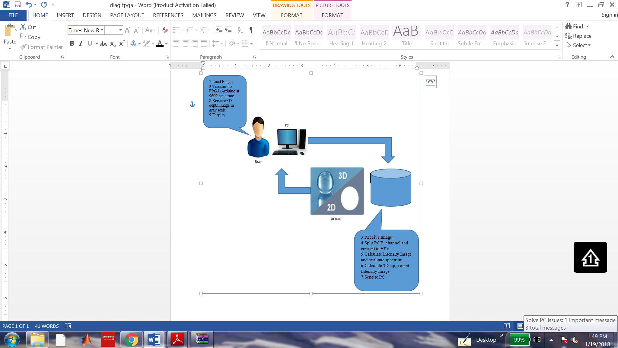Figure 2. Block diagram of process

Since Papilio One is used for conversion and it has memory constraint ,instead of whole image being sent at a time to the kit, serially pixels are sent to Papilio One for computation one row after another. HSV image is then generated in MATLAB from these processed pixels.

2.3.  Edge detection

As per Figure 1 the next step is to detect the edge. Here the input images are converted to gray scale for proper edge detection. Edge detection is the technique of identifying those points in the digitized image which causes a drastic change in the splendor of the image or that causes discontinuities. The edges are identified by rapid change in frequency.  The objective is to capture these much needed rapid variations in the properties of the world. Edge detection is done by applying masks on the input which transforms the image into output image highlighting the sharp edges in the object. There are several masks available like Canny, Prewitt, Sobel, Roberts etc. which extracts the sharpness in the images.

The Canny detection is a popular edge detection method. It basically locates the maxima of gradient-I in the neighborhood.    Gaussian channel derivative is used to compute the gradient. All the four steps [9] are used to detect the edges of the image. The strategy utilizes two edges, to distinguish solid and frail edges, and incorporates the powerless edges in the yield just on the off chance that they are associated with solid edges. Gaussian channel is connected to evacuate any clamor show in a picture, and more inclined to identify genuine powerless edges [10].

Object should be detected properly, because if it is not then the next operation of hole filling will not be performed properly. Morphological dilation operation is added before the hole-filling to improve the object detection. Pixels are added to the object boundaries during dilation and the number of pixels added is a function of the shape & size of the structuring elements deployed for processing the image.

2.4.  Hole filling and depth estimation

The images under go morphological operations viz., dilation  and after dilation operation, the detected objects are  filled using MATLAB imfill function. For this  filling operation  first labeling is done using `bwlabel’ function which generates a matrix same size as that of the input matrix containing labels for all connected objects in the input matrix.

The input “n” can either be a four connected or eight connected objects with a default value of eight. The pixels with 0 labelling coressponds to the  background and the labelling from 1 through 8 coressponds to each of the coneected objects. The ouput gives the number of the connected objects in the iput image. Along with bwlabel function  n is used to return vectors of indices for the pixels that make up a specific object. Then that specific object is cropped for  filling new depth values using `imcrop’ function. This function creates an interactive crop image. From that cropped object maximum and minimum values are calculated. For the same coordinates, values of V (intensity) retrieved from FPGA are stored in array. From the array maximum and minimum values of V are searched to calculate the range. 255/range = multiValue. So for the same coordinates the new value which gives depth is calculated using following equation:

val=((imgHSV(yy,xx,3))-minVal)*multiVal                        (1)

where, val is new depth value of depth, (imgHSV(yy,xx,3) gives values of V for that particular pixel, minVal is minimum value from array and multivalue .

2.5.  Anaglyph Image Generation

So far depth map image is estimated, now using this depth map and 2D input image anaglyph image is generated. The anaglyph image is generated by using the difference value of each pixel from the depth map. Each pixel is shifted by the corresponding difference value in an input image. The parallax is given by

parallax(x,y)=C[1-depth(x,y)]/128                                       (2)

where C is the maximum parallax.  Anaglyph image is got by shifting each pixel to the right by parallax(x,y)/2.

Algorithm:

• Load input 2D image from database.
• Send input images pixel serially to FPGA to perform RGB to HSV conversion.
• Display HSV image on PC.
• Convert input image to grayscale image.
• Perform Canny edge detection on grayscale image.
• Display edge detection output.
• Perform dilation operation on edge detection output.
• Perform hole filling operation.
• Label images for object detection.
• Crop the detected objects.
• From the HSV image get the values of V for the same coordinates of the object.
• Assign depth value to new pixel using equation 1 and display.
• Generate anaglyph images and display.

3. Simulation Results

The algorithms we used work only for restricted scenario since cues are not considered. Proposed algorithm is tested for indoor image database, outdoor images database and database created by our own. Figure 3 is the output of various stages of proposed block diagram.

Input is from Make3D dataset of 500X 500 resolution. The first dataset used is a Make3D dataset made up of out-door images which has the depth fields that are acquired by a laser finder. For computational efficiency, the images are resized and the resolutions of the Make3D images are 1704 x 2272. All the stages of the block diagram are given as the output. Figure 3 (f) gives the 3d output which has to be viewed by the 3d glasses.

Figure 4 is the output of various stages and Input is from Middlebury dataset of 300X 259 resolution an in-door image, for computational efficiency, the images are re-sized. Figure 4 (f) gives the 3d output which has to be viewed by the 3d glasses.

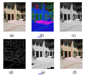Figure 3: (a) Query  (b) HSV (c) Grayscale  (d) Edge Detected (e) Depth (f) Anaglyph .

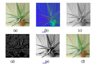Figure 4: (a) Query (b) HSV (c) Grayscale (d) Edge Detected (e) Depth (f) Anaglyph.

We continued the experiment with our own database with dataset of 300 X 225 resolution, indoor images. The quality of the output was good as that of the Middlebury.

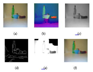Figure 5: (a) Query (b) HSV (c) Grayscale (d) Edge Detected (e) Depth       (f) Anaglyph

 Following is the analysis of the images in terms of computing time efficiency of Make 3D dataset. The algorithm was executed in MATLAB and in FPGA and the table shows the time taken of the images for execution.

Table 1: Analysis of Images from Make3D Dataset

Size of input image	Execution time
	MATLAB	FPGA
100*100	1.08ms	15min 26s
200*200	1.76ms	1hr 00min
300*300	9.05ms	2hr 26min
400*400	37.41ms	4hr 06min
500*500	122.65ms	–
600*600	274.75ms	–
700*700	505.38ms	–
800*800	888.00ms	–
900*900	1451.07ms	–
1000*1000	2196.97ms	–

The time taken by MATLAB to execute the complete process using a single core processor is in milliseconds and for FPGA the time taken is exponentially increasing with increase in the size of the input image. For any real time processing MATLAB would give a time efficient output and the future scope is to extend this algorithm work for multi-core processors.

4. Subjective analysis

Various objective quality metrics like MSE and PSNR are available. This can be used for objective analysis of 2D but not suitable for the 2-D to 3-D contents [11]. The generated depth-map is a pseudo-depth map and is not a real depth-map. So to evaluate the visual quality of output of proposed algorithm it is compared with other algorithms [12]. Figure 6 shows the form shared with people to mark the quality of the images shared with them to analyze. It shows the credit score in percentage depending on the visual perception of the viewer.

Figure 7 shows the subjective analysis of people. For subjective analysis survey from 50 people with normal or correct-to-normal visual acuity and stereo acuity for visual comfort of output. We have shown them output of our algorithm and for the same images output of other two methods.  Images are taken from standard dataset.

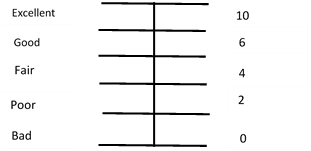Figure 6: Rating scales used for assessment

Table 2 shows subjective evaluation, where M1 is our method, M2 is global method and M3 is Make3d algorithm. People has given good scale to our algorithm while excellent scale to other to algorithms. The scale on which people has given rating is shown in Figure 6. From the survey its found that they felt proposed methods output good, while of other two method’s excellent. The subjective analysis also shows that proposed algorithm provides comfortable viewing experience.

Table 2: Sample Analysis of Images from Make3D Dataset

viewer count	Image1			Image 2			Image 3			Image 4
	M1	M2	M3	M1	M2	M3	M1	M2	M3	M1	M2	M3
1	8	10	10	8	10	10	8	10	8	6	10	8
2	6	10	10	6	10	10	8	10	10	6	10	10
3	8	10	10	6	10	10	8	10	8	6	10	8
4	8	10	10	8	10	10	8	10	10	8	10	10
5	8	10	10	8	10	10	8	10	10	6	10	10
6	8	10	10	8	10	10	8	10	8	8	10	8
7	8	10	10	8	10	10	8	10	8	8	10	10
8	8	10	10	8	10	10	8	10	8	8	10	10
9	8	10	10	8	10	10	8	10	8	8	10	8
10	10	8	8	10	8	8	8	10	8	8	10	8
total	80	98	98	80	98	98	80	100	86	72	100	90

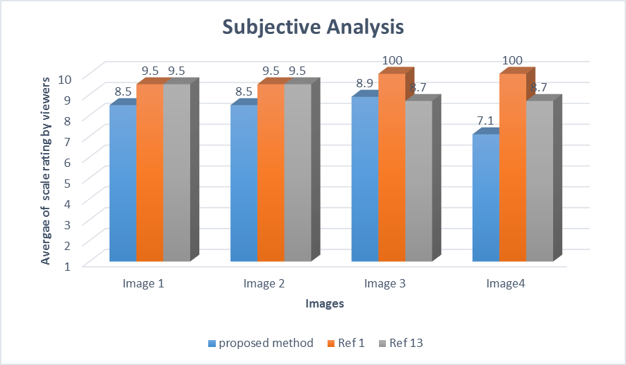Figure 7: Graph of Subjective Analysis

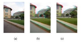Figure 8: output images (a) proposed method (b) global  method  (c) Make3d

5. Conclusion

        In current scenario, 2D-to-3D conversion is a very active research area as it gives more lifelike viewing experience and hence its popularity is increasing. As there are many hardware available which support 3D and hence there is an urgent need of 3D contents. Though there are distinct methods introduced by researchers but these method works for restricted scenes.

In this paper 2D-to-3D image conversion was implemented which can take global image as an input. The work comes under automatic approach of conversion, in which algorithm itself does the whole conversion. Using RGB to HSV conversion along with simple MATLAB operations 2D image is converted into 3D. The method was tested on three distinct standard databases and on our own database. For output analysis subjective evaluation was done on 10 people for visual comfort of implemented systems output with the output of other two methods. People rated output as good from scaling range as visual comfort.

The work can be further extended by working on video. Here conversion from RGB to HSV step is implemented on starter kit of FPGA; it may be possible to implement whole system on a computational efficient FPGA.

Conflict of Interest

The authors declare no conflict of interest.

Acknowledgment

The authors hereby express their gratitude to Dr. D Y. Patil Institute of Engineering, Research and Management, Akurdi for facilitating this research.  We are highly privileged to have got the much needed support and assistance from almost each and every people of the institution for the successful outcome of this work.  Special thanks, to all the teaching staffs of the institution, for their constant encouragement and guidance which has helped us in successfully completing this work. .

1. Phan and D. Androutsos “ Literature survey on recent methods for 2d to 3d video conversion” Multimedia Image and Video Processing, Second Edition, pages 691to716, 2012.
2. Konrad, Meng Wang, P. Ishwar, Chen Wu, and D. Mukharjee. “Learning-based, automatic 2d-to-3d image and video conversion”. Image Processing, IEEE Transactions on, 22(9):3485-3496, 2013. https://doi:10.1109 / TIP. 2013.2270375.
3. Pan Ji, Lianghao Wang, Dong-Xiao Li, and Ming Zhang. “An automatic 2d to 3d conversion algorithm using multi-depth cues”, In Audio, Language and Image Processing (ICALIP), 2012 International Conference on, pages 546-550, 2012.
4. Guttmann, L. Wolf, and D. Cohen-Or. “Semiautomatic stereo extraction from video footage” Computer Vision, 2009 IEEE 12th International Conference on, pages 136-142, 2009.
5. Make3D, Convert your still image into 3D model, (2015, June 20). http://make3d.cs.cornell.edu/data.html.
6. NYU Depth Dataset V2, (2016, Jan 11) , https://cs.nyu.edu/ ~ silberman / datasets /nyu_depth_v2.html
7. Middlebury Stereo Datasets,  (2013, Nov 14), http:// vision.middlebury.edu /stereo/data/
8. Welcome to Sony Support , (2015, Dec 24),  https:// www.sony.co.uk /electronics /support
9. Zhao Xu1, Xu Baojie, Wu Guoxin1 “Canny edge detection based on Open CV” 2017 IEEE 13th International Conference on Electronic Measurement & Instruments ICEMI’, pages 53-56, 2017.
10. Janusz Konrad, Meng Wang, and Prakash Ishwar,” 2D-to-3D Image Conversion by Learning Depth from Examples”, Computer Vision and Pattern Recognition Workshops (CVPRW), 2012 IEEE Computer Society Conference, 2012. https://doi.org/ 10.1109/CVPRW.2012.6238903.
11. Mani B. Fard, Mani B. Fard, Ulug Bayazit, Ulug Bayazit, “Automatic 2D-to-3D video conversion by monocular depth cues fusion and utilizing human face landmarks”, Proc. SPIE 9067, Sixth International Conference on Machine Vision (ICMV 2013), 90670B, 2013. https://doi.org/10.1117/12.2049802.
12. Saxena, A. and Min Sun and Ng, A.Y. Make3D:” Learning 3D Scene Structure from a Single Still Image”. Pattern Analysis and Machine Intelligence, IEEE Transactions, pages 824-840,2009.https://doi.org/ 10.1109/TPAMI.2008.132.

(Click Here)

(Click Here)