1. Introduction

With the popularity of mobile location devices, the acquisition of location information is becoming more and more easier. Location-based services have become common services in our lives. It is necessary for us to mine location data and use the acquired knowledge to extend location services or improve service quality. Location prediction is an important research point in the field of location data mining, which can provide us with better recommendation services, social networking services and so on.

This paper is an extension of work originally presented in conference name [1].

Markov chain is a set of discrete random variables with Markov and the probability of each event depends only on the previous event. The Markov process is named after the Russian mathematician Andrey Markov. In this process, the future state is only related to the current state and has nothing to do with the past. Markov chain is divided into continuous Markov chain and discrete Markov chain. In discrete state-space, discrete time random process is called discrete Markov chain, and continuous time random process is called continuous Markov chain. [2]

Markov chain is a common statistical model, which is widely used in various kinds of prediction. It has the advantages of simplicity and efficiency, and is a good representation of time series data. Therefore, it can also be used for location prediction.

In literature [3], a location prediction method based on adaptive higher-order Markov model was proposed, which significantly improves the accuracy of location prediction. The difference between a higher-order Markov model and a Markov model is that the future state depends on the current state of the model and the past k-1 state of the model, not just the current state. However, it does not solve the problem of not finding current state in the history data, which is called the zero frequency problem. Literature [4] used variable-order Markov model for location prediction. It is based on high-order Markov model and makes the best use of history data. The zero frequency problem is also solved by an approach called escaped rule. Moreover, we found that many people have a regular life activity. By analyzing these people’ history data, certain rules can be mined in time and space. These rules can be used in location predication. In the literature [5], the author not only considered the influence of user space factors on location prediction, but also considered the time factor, which further improved the accuracy of location prediction. This lets us notice the importance of time factor in location predication. Literature [6] provided a method for location prediction by using space-time rules, which is not only simple, but also can obtain good prediction results. These studies gave us a lot of inspiration.

With lots of studies, a location predication method based on variable-order Markov model with time feature and user’s spatio-temporal rule was proposed. It included the preprocessing of data, the construction of variable-order Markov model with time feature and the analysis of the time and spatial rules of users. First, data preprocessing makes the location data more suitable for location prediction. Since time and spatial factors both have impact on location predication, a variable-order Markov model with time feature is constructed for location predication. Finally, for the case that the variable-order Markov model cannot be used to perform the prediction, the prediction is made by analyzing users’ time and spatial rules.

2. Data preprocessing

Before predicting the location, location data needs to be preprocessed, which includes three steps, that is, data cleansing, location information abstraction and stay point extraction.

2.1.  Data cleaning

The purpose of data cleansing is to make the data more real, regular, and easy to handle. First, you need to modify the irregular data to make it more regular. Second, data not in research range needs to be deleted. In this study, Beijing was chosen as the research object so the range of location data control is between east longitude 115.25 ˚ to 117.3 ˚ and north latitude 39.26˚ to 41.03˚. If not, it is regarded as data that is not in this range. Finally, incomplete or unreal data are cleaned up.

2.2.  Location information abstraction

Location data is usually obtained by mobile device. And it is mainly composed of coordinate location data. The data are very detailed and it is difficult for us to analyze them. Location data needs to be abstracted into area data to perform conventional mining. The abstraction of location data also helps decrease computational complexity. In literature [7], the idea of building active grid was proposed. We use this method to abstract the location data:

• First, the user’s activity range is set in a large rectangular area and the edge is parallel to the longitude and latitude lines.
• Then, the rectangular area is divided into a square grid. And the user’s location point is mapped to the grid.
• Finally, active grid is connected based on time passage. This is user’s active grid sequence.

The raw location data is composed of points. This is original trajectory data. {p₁,p₂…p_i…p_n}. P_i is the location point in the trajectory data. After the abstraction, the original user location sequence {p₁,p₂…p_n} is converted to active grid sequence {z₁,z₂…z_i…z_n}. z_i is the grid in the abstract trajectory data.

2.3.  Stay points extraction.

The stay points of moving objects are important points or areas such as shopping centers, workplaces, places of residence and so on. These points should be emphasized in location-based services. Therefore, the stay points in the trajectory need to be extracted. And there are many ways to extract stay points. The method of considering time and space factors is not only simple but also effective. It is based on the principle that a place is a stop point when you stay longer than the set time. The extraction method includes the following steps:

• Set the time value t, which is the standard of residence time.
• Search the area with residence time exceeding t in the trajectory data. The residence time is calculated by the difference between the maximum residence time and the minimum residence time.
• The stay points by time chronological order constitutes the new track.

The trajectory data composed of residence points are extracted by the above method. Algorithm 1 is the pseudocode used for the residence point extraction.

Algorithm 1 Stay points extraction

Input: User’s historical data d_data  and stay time threshold t Output: User’s stay points s_area The maximum time value to stay in the area time_max The Minimum time value to stay in the area time_min Sort the data of d_data by time for each area of  d_data do stay time = time_max -time_min if stay time > t The area  add to the stay area s_ area end for

return s_ area

3. Location Prediction

The method of location prediction includes constructing variable-order Markov model with time feature and analysis of user’s time and spatial rules. It’s named location prediction based on variable-order Markov model with time feature and user’s spatio-temporal rule (VMTST).

3.1.  Variable-order Markov Model with Time Feature construction and prediction methods

Variable-order Markov model is an improved model based on high-order Markov model. It makes use of the excellent prediction ability of the high-order Markov model and further realizes the automatic selection of high-order Markov model order. Time feature are also important for location prediction. Thus, time feature and variable-order Markov model are combined, and the scoring method is used to achieve the location predication. The method is as follows:

• Extract the historical track data composed of user’s stay points.
• Search history tracks based on the user’s current track. If the matching historical trajectory information is found, the transition probability of the next grid in these trajectories is calculated. It is called
• If the matching track information is not searched, some active grids must be removed and then new current track is created. The earliest active grids need to be removed because the earlier an active grid arrives, the less impact it will have on its future location. This process requires multiple executions until matching trajectory data is found.

For example, Figure 1 shows the user’s historical trajectory. If the user’s current trajectory (Z₂-Z₃), all historical trajectory data containing (Z₂-Z₃) are searched. Z₄ after calculation is the highest region with transition probability. Region Z₄ is the predicated result. But if the user’s current trajectory is (Z₄-Z₅-Z₆). The current trajectory is not found in history data. Z₄ is the earliest region and has the least influence on location predication, so Z₄ region should be deleted and search it again from the historical track.

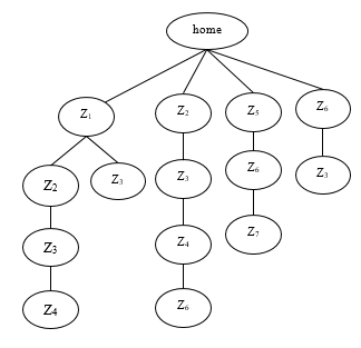Figure 1: User’s historical trajectory

• For each candidate region, their scores are composed of spatial accessibility scores and time feature scores. The scoring formula is as follows:

W₁ and W₂ are the weights which are possible to reach spatial scores and time characteristic scores in the total scores.

Time information includes two parts: date and time. Therefore, the score of time feature S is composed of two parts: the periodic coefficient of the date and the similarity score of time.

Si is the similarity score of time. Clustering and normalization idea is used here. It is obtained by the following formula.

th is the hourly portion of historian data record.

tn is the hour component of current status.

C is the periodic coefficient of date. It is divided into workdays and holidays. It is calculated by the following rules:

If record date and forecast date are workdays, it means the location data is regular. Thus, the value of C is greater than 1.

If historical date and forecast date are holidays, it means the location data is irregular. Thus, the value of C is less than 1.

In other cases, C is 1 .

• The zone with the highest score is used as the predicting outcomes.

The location prediction algorithm of variable-order Markov model with time feature is as follows:

Algorithm 2 Construction of the variable-order Markov model with time feature

Input: users historical data h_data,users current trajectary c_try Output: users next area n_zone The weight of the space in the total score W1 The weight of the time in the total score W2 while Search from historical data (h_data) with user’s current trajectory(c_try) return false c_try = remove the earliest zone from the user’s current trajectory if the number of areas in user’s current trajectory ==1 break Calculate the transition probability P of each next areas in the matched trajectory for each area of next areas do Calculate the time similarity score Si and date coefficient C for this area Time feature score for this area S = C*Si Score for this area score = W1*P+W2*S end for Search for the highest scored area n_zone in the next area of historical data return n_zone

3.2.  Analyze Spatio-temporal Rule of Moving Objects

When users have less historical data, it is difficult to search matching historical track information. Location predication is done by analyzing the user’s time and spatial rules. Spatio-temporal rule mainly refers to the regularity of users’ time and spatial positions at different times. The following methods are used to analyze the spatio-temporal rule of users:

• The time interval is set to t.
• In the user’s historical data, count the number of occurrence of user in each interval and each active grid. The region with the maximum number is the hot spot region during this time period.
• Set the numbered ID for each time period in time order.
• The result of spatio-temporal rule is composed of ID, hot region.

During this period, the more time periods are divided, the better the prediction effect is, but the more time is needed for calculation. It is easy to understand that the more active grids are present, the more likely they are to become a mobile destination for users. Therefore, hot spot active grids with the maximum number of occurrences are the prediction area based on spatio-temporal rule. Algorithm 3 describes this process.

In the location prediction, the user’s current activity time matches the ID in the spatio-temporal rule. Next ID hotspot region is searched in the spatio-temporal rule, which is considered a place where users may arrive in the future. This process is algorithm 4.

Algorithm 3 Analysis of user’s spatio-temporal rule

Input: users historical data h_data, time period t

Output: users spatio-temporal rule result s_t_result Dividing the time period according to the value of t for each time period do Set a number for each time period t_ID Calculate the area with the most user arrivals during this time period max_area t_ID and max_area added to the spatio-temporal rule result s_t_result end for return s_t_result

Algorithm 4 Location prediction using user’s spatio-temporal rule

Input:users spatio-temporal rule result s_t_result recording time of the user’s current trajectory r_time Output:location prediction area obtained by users spatio-temporal rule next_area Get the number of the r_time named n_ID for each number in the time period do  if n_ID = number in the time period get the hot area of the next time period hot_area next_area=hot_area return  next_area

4. Experiment

4.1.  Experimental design

In order to verify the effectiveness of the proposed prediction method, experiments were performed using the GeoLife [8] trajectory data set. This data set includes trajectory data of 182 users over five years. It has about 18,670 tracks, including longitude, latitude, time and other information. And it records track data like users’ work, entertainment and sports as well as other outdoor activities.

After data cleansing, extract the user’s ID, longitude, latitude, date, time and other attributes. The experiment data set is shown in table 1. 10% data is randomly selected for test data and the rest are training data. Experimental research area is east longitude 115.25˚ to 117.3˚ and latitude 39.26˚ to 41.03˚. The size of grid unit is 100m*100m, the limit time of residence time point t is 10 min and the time interval selected for the analysis of users’ spatio-temporal rule is 2 hours.

Contrast model:

MM: High order Markov location predication model.

VOMM: Location prediction model proposed in literature[4] uses variable-order Markov model for location prediction and escaped rules to solve the zero frequency problem.

VMSTPM: The location prediction model is proposed in literature [1]. This method uses the variable-order Markov model for location prediction and also uses spatio-temporal rule to solve the zero frequency problem.

Table 1: Sample of Data

ID	latitude	longitude	date	time
10	39.921695	116.472345	2007-08-04	03:30:34
10	39.961675	116.472315	2007-08-04	03:30:36
10	39.924583	116.472290	2007-08-04	03:30:38
10	39.921572	116.472290	2007-08-04	03:30:39
10	39.921565	116.475588	2007-08-04	03:30:40
10	39.921577	116.472210	2007-08-04	03:30:41
10	39.921570	116.472300	2007-08-04	03:30:42
10	39.921576	116.475588	2007-08-04	03:30:44
10	39.921580	116.472290	2007-08-04	03:30:46
10	39.921576	116.472321	2007-08-04	03:30:50

4.2.  Evaluation Factors

Prediction accuracy and recall rate were used as evaluation indexes in the experiment. The formula is as follows:

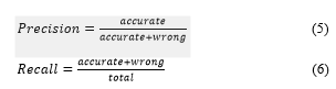Table 2: The value of W₁ and W₂ in different situation

	case 1	case 2	case 3	case 4	case 5	case 6	case 7	case 8	case 9
W1	0.1	0.2	0.3	0.4	0.5	0.6	0.7	0.8	0.9
W2	0.9	0.8	0.7	0.6	0.5	0.4	0.3	0.2	0.1

Table 3: The value of C₁ and C₂ in different situations

	case 1	case 2	case 3	case 4	case 5	case 6	case 7	case 8	case 9
C1	1.1	1.2	1.3	1.4	1.5	1.6	1.7	1.8	1.9
C2	0.9	0.8	0.7	0.6	0.5	0.4	0.3	0.2	0.1

In the above equations, accurate indicate the number of correct predictions, wrong indicate the number of incorrect predictions total indicate the number of all testing trajectories.

4.3.  Analysis of Experimental Results

First, the coefficients in the candidate region scoring formula were tested by experiments and prediction accuracy was used as the evaluation index. The experiment selected nine different values, as shown in table 2. From table 2, we can see that the prediction accuracy is the highest when W₁ and W₂ are 0.3 and 0.7. It proves the importance of time feature to location prediction. Thus, when the weight of time feature is great, the prediction accuracy is higher.

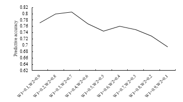Figure 2: Prediction precision of W₁ and W₂ in different situations

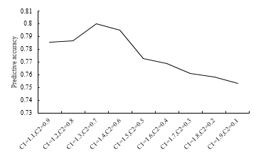Figure 3: Prediction precision of  C₁ and C₂ in different situations

Besides, the period coefficient value of the date obtained the best value by experiments. The value of C is C₁ when record date and prediction date are both workdays. And the value of C is C₂ when both historical date and prediction date are holidays. C₁ and C₂ take the values in table 3. It can be seen from figure 3 that the prediction outcome is best when C₁ is 1.3 and C₂ is 0.7. Therefore, other experiments were performed with these values.

Then, lots of prediction experiments were performed to verify the prediction outcome of the model. The prediction outcome is shown in figure 4. And VMTST at different orders showed more accurate prediction result. The best prediction result is obtained in the second order, which is about 30% higher than the original high-order Markov model and about 20% higher than the VOMM model. In figure 5, we can see that VMTST model is more stable in higher-order predictions. Therefore, it is better to use the current state and a history state for location prediction. This will get the optimum result. These results show that VMTST model has good predictive performance.

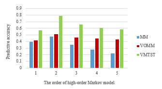Figure 4: Prediction precision with different orders

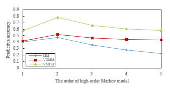Figure 5: Prediction precision with different models

Experiments were conducted to verify the importance of time in prediction. The prediction accuracy is still used as the evaluation index in the experiment. And the results are shown in figure 6. It can be seen that the prediction accuracy of VMTST is higher than that of VMSTPM with different orders, which proves that time feature is a very important factor in location prediction.

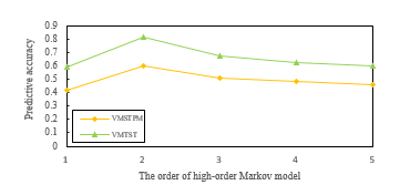Figure 6: Prediction precision of VMSTPM and VMTST

The figure 7 is the comparison of recall rates of three models. As you can see, the recall rate of VMTST is 1.0, which is higher than high order Markov model. This means that it is effective to solve the zero frequency problem by using the user’s spatio-temporal rule. However, the recall rate of VOMM model is also 1.0, which means VOMM model also solves the zero frequency problem. More experiments are required to verify the performance of VMTST.

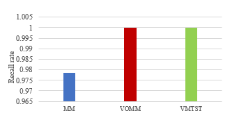Figure 7: Recall rate of different models

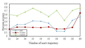Figure 8: Prediction precision of users with fewer trajectory

The above experiments show that the spatio-temporal rule can solve the zero frequency problem. But, it is necessary to verify the performance of spatial and temporal laws in predicting accuracy through experiments. The experiment selected 10 users with less historical data. Therefore, it is easier to generate zero frequency problem. And it can be seen from the experimental results in figure 8 that when the trajectory quantity is small, the prediction accuracy of VMTST model is still higher than other models. Therefore, the spatio-temporal rule of users is more suitable to solve the problem of zero frequency.

5. Conclusion

A location prediction method was proposed in this paper, including preprocessing of location data, construction of variable-order Markov model with time feature and analysis of user’s spatio-temporal rule. The preprocessing of position data makes the research scope fixed and the track data easier to analyze and process. Variable-order Markov model is an improved model of high-order Markov and it has higher location prediction accuracy. The time features are added to the variable-order Markov model to further increase the prediction accuracy. The problem of zero frequency can be solved by analyzing the spatio-temporal rule of users. Finally, lots of experiments were carried out using the actual trajectory data set.

By summing up the experiments, we can conclude that VMTST model improves the prediction accuracy. Time features are very important for location prediction. And the spatio-temporal rule can solve the problem of zero frequency, and be also more suitable.

In the future, we will look for new methods to mine the spatio-temporal rule of users so as to get the higher prediction accuracy. Also we will study the application of location prediction method in practice.

1. Y. Xia, Y. Gong, X. Zhang and H. Y. Bae, “Location Prediction Based on Variable-order Markov Model and User’s Spatio-temporal Rule” in International Conference on Information and Communication Technology Convergence, Korea, 2018. https://doi.org/10.1109/ICTC.2018.8539593
2. P. A. Gagniuc, Markov Chains: From Theory to Implementation and Experimentation, John Wiley & Sons, 2017.
3. M. Q. Lü, L. Chen, G. C. Chen, “Position Prediction Based on Adaptive Multi-Order Markov Model” Journal of Computer Research and Development, 47(10), 1764-1770, 2010
4. J. Yang, J. Xu, M. Xu, N. Zheng, Y. Chen, “Predicting next location using a variable order Markov model.” ACM Sigspatial International Workshop on Geostreaming, USA, 2014. https://doi.org/10.1145/2676552.2676557
5. X. Li, C. Yu, L. Ju, J. Qin, Y. Zhang, L. Dou, S. Y. Qing, “Position Prediction System Based on Spatio-Temporal Regularity of Object Mobility” Information Systems, 75, 43-55, 2018. https://doi.org/10.1016/j.is.2018.02.004
6. H. M. Wong, S. V. Tseng, C. C. J. Tseng. “Long-Term User Location Prediction Using Deep Learning and Periodic Pattern Mining.” in International Conference on Advanced Data Mining and Applications, 2017. https://doi.org/10.1007/978-3-319-69179-4_41
7. F. Giannotti, M. Nanni, F. Pinelli, “Trajectory pattern mining.” in Acm Sigkdd International Conference on Knowledge Discovery & Data Mining ACM, 2007. https://doi.org/10.1145/1281192.1281230
8. Y Zheng, X Xie, W. Y. Ma, “GeoLife: A Collaborative Social Networking Service among User, location and trajectory” IEEE Data Eng, 33(2), 32-39, 2010

(Click Here)

(Click Here)