1. Introduction

This study focuses on traffic flow and congestion analysis especially in the under developing country (India). In the previous study,  it is proposed the traffic service quantitative traffic congestion analysis method in the International Conference on Advances in Computing, Communications and Informatics (ICACCI) [1]. From the actual measurement traffic data study during more than one month in Ahmedabad city of Gujarat State in India, the major traffic parameters are extracted from the traffic fundamental diagram such as traffic density (k) to vehicle average speed (v) and traffic density (k) to traffic volume (q), which introduced at the International conference CODATU 2017 [2].

As for obtaining the traffic parameters and analysis, the detail  is explained in the next section. The previous study of CODATU introduces the unique traffic characteristics  which is useful for using Envelopment Observation method because there is clear boundary in those characteristic and it is appropriate way to define the traffic parameters from their unique measurement data. The another phenomenon from the measurement data is vehicle speed ratio which is the ratio of average vehicle speed (v_ave) to free speed (v_f). The value of this speed ratio (SR) is valid for understanding congestion level of each road. When S.R. becomes lower than 0.65, the condition of road becomes congested. Author found similarity of this phenomena between the Indian traffic flow model and viscous fluids model between parallel flat plates.

In this extension of the research,  more detail analysis is added between SR and occupancy of traffic parameter which is used as traffic congestion level judgement from traffic engineering. In addition, the relationship between parameter occupancy and traffic density is described in order to understand traffic congestion condition. As for the traffic congestion analysis, it also describes the time zone base analysis in this paper. From this time zone base analysis, we found there are two patterns for Ahmedabad traffic congestion condition. One is heavy traffic density congestion which follows the traffic flow theory and the other is unheavy traffic density congestion which is unique in India. Therefore it is important for considering what is the traffic congestion definition. when the traffic information is provided from the traffic information sign board so called VMS or Various Message Sign on the road.

2. Related Studies

2.1.  Traffic Flow Theory and Measurement Analysis of Ahmedabad city

In the previous study for Ahmedabad traffic flow analysis at CODATU conference, the traffic fundamental diagram is introduced such as k–v curve (traffic density (k) to average vehicle speed (v)), k–q curve (traffic density (k) to traffic volume (q)), and q–v curve (traffic volume (q) to vehicle speed (v)). This analysis has been continued since Ahmedabad ITS or Intelligent Transport Systems business project from October 2014. The project is providing Ahmedabad city to provide its traffic condition for the drivers through VMS. The ITS system consist of four VMSs and 14 traffic monitoring cameras. The traffic flow condition is captured by the traffic monitoring cameras and its result of analysis is shown at the VMS for considering change route or using other transportation choice. The Ahmedabad ITS system configuration is shown Figure 1.

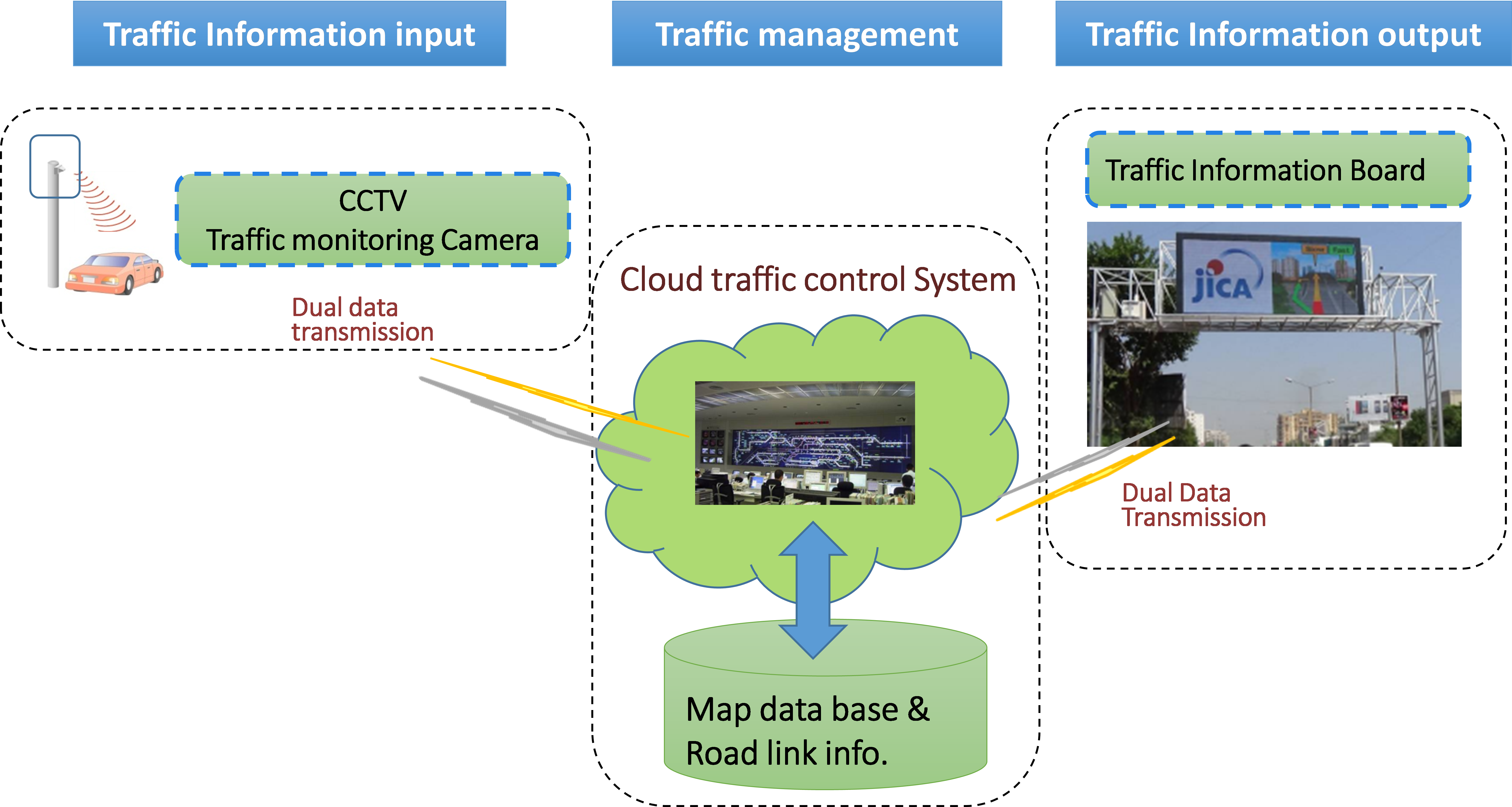Figure 1: Ahmedabad ITS system configuration

In the CODAU study, authors found the unique characteristics of Ahmedabad traffic flow measurement data. There is clear boundary in each traffic fundamental diagram. The k–v curve and k–q curve at Camera#1 are shown in Figure 2.

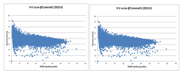Figure 2: Traffic Flow Characteristics at Camera#1

From Figure 2, there is clear boundary in each characteristics curve by envelop observation.  The other characteristics at other location are similar results which are omitted in this paper. When these boundary are taken as traffic flow characterizes, it is able to adjust traffic flow characteristics curve from traffic flow equation to the envelop line. The Figure 3 shows the example of adjustment result between traffic flow theoretical curve from its equation and the measurement data at Camera#1.

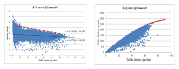Figure 3: Traffic Flow Characteristics at Camera#1

In terms of traffic equation form the theory, traffic density (k) to traffic speed (v) equation is given by (1) and traffic density (k) to traffic volume (q) equation is given by (2). The equation (1) is so called Greenshields [3] curve.

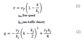The theoretical curve illustration is shown in Figure 4.

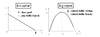Figure 4: Theoretical Traffic Flow Curve

In the advanced country traffic flow, the actual measurement plots including Japan [4] are aligned with theoretical curve and or near boundary in Figure 4.  Therefore the traffic characteristics curve from measurement in Ahmedabad is quite different from those of the advanced countries (refer to Figure 2).

2.2.  Quantitative Traffic Congestion Study in Ahmedabad

The traffic congestion problem in developing countries become more serious situation these days, especially in India. Therefore it is crucial to establish for analysis method about the traffic congestion quantitatively. In the International Conference on Advances in Computing, Communications and Informatics or ICACCI, T.Tsuboi proposes quantitative traffic congestion analysis based on the actual traffic measurement in Ahmedabad. In this paper, it is introduced the traffic congestion by vehicle speed ratio (SR) which is the ratio of the average vehicle speed (v_ave) to the free speed (v_f). In ICACCI paper, it is defined that the threshold level of traffic congestion is 0.65. The comparison SR at each traffic camera location is shown in Figure 5. According to Figure 5, the Camera#2 is most small value. And the actual daily traffic flow (traffic volume and average vehicle speed) at Camera#2 in June 2015 is shown in Figure 6 (a) and (b). From Figure 6(b), the average vehicle speed is lower than 20km/h, which shows the traffic congestion occurred [5].

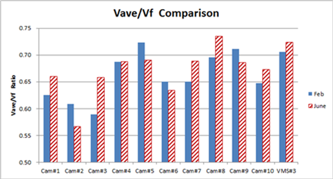Figure 5: Traffic Speed Ratio Comparison in Ahmedabad

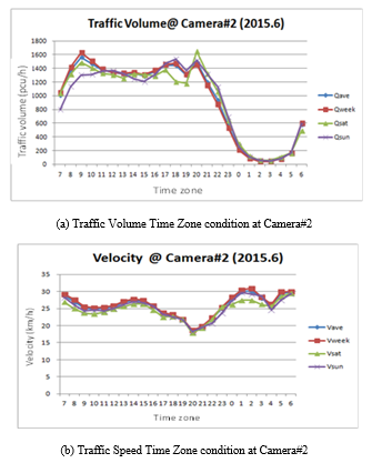Figure 6: Daily Traffic Flow condition at Camera#2

From Figure 6 (b), it is a clear difference that Camera #2 vehicle velocity ratio is lower than other locations. According to traffic flow theory, most of measurement data of q–k curve is located at shadow area in Figure 7. And free traffic flow area is bottom part of q – k curve; jam traffic flow area is top of q – k curve. But our measurement data of q – k curve in Camera # 2 is located inside q – k curve (refer to Figure 7). The speed ratio of inside curve area is lower than 0.65 which means that its traffic condition becomes congested.

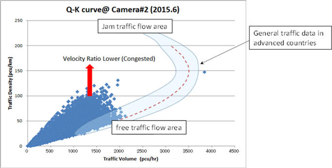Figure 7: q – k Curve at Camera#2

In order to identify that inside curve area is under congested condition, we divide between two areas. One area has speed ratio equal and less than 065 and the other area has speed ratio more than 0.65. Figure 8 shows those two areas. According to Figure 8, the speed ratio equal and lower than 0.65 (≈ 2/3) is inside envelope line area. According to the previous traffic flow analysis, the threshold   between free flow and congested flow occurs at the average vehicle velocity (v_ave) ≤ 2(v_f) /3 [2]. Therefore the traffic flow capacity is able to obtain by our envelope data analysis and it is able to be described by the traffic flow equation. This is the first time to show emerging countries traffic analysis and brings basic traffic flow parameters by boundary traffic analysis. And vehicle velocity ratio of average speed by free speed is good reference of explaining traffic jam condition; the critical value of speed ratio is 0.65 in this paper.

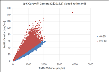Figure 8: q – k measurement data by vehicle Speed Ratio at Camera#2

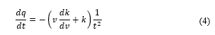
In terms of traffic congestion analysis, the congestion social loss analysis theory [6] is used. From the traffic flow theory, traffic volume (q) is mathematical product by vehicle velocity (v) multiplying to traffic density (k) shown in (3).

Since the vehicle velocity (v) is inverse of travel time (t), then the vehicle velocity is described as v = 1/t.  Therefore traffic volume (q) is a function of travel time (t). Assuming that the traffic user’s opportunity n per unit time is constant, travel time (t) is proportional to the cost of traffic congestion. In another word, the relationship between traffic volume (q) and travel time (t) means the traffic supply curve of the relationship between traffic service supply and cost. In order to analyze traffic volume (q), differentiating e (3) by (t) provides (4).

When vehicle velocity (v) becomes large volume (travel time becomes small value), traffic density (k) becomes small value and then dk/dv < 0. Therefore he value in parenthesis of (4) is negative and then dq/dt becomes positive value. This relationship is illustrated in Fig.8. The supply curve line rises to the right from travel time (1/v_f) to (1/v_c), which means private cost curve for transportation. And when (v) becomes small value (travel time (t) becomes large value), the value in parenthesis of (4) becomes positive and the supply curve drops to the right, which corresponds to private cost curve drops to the right.

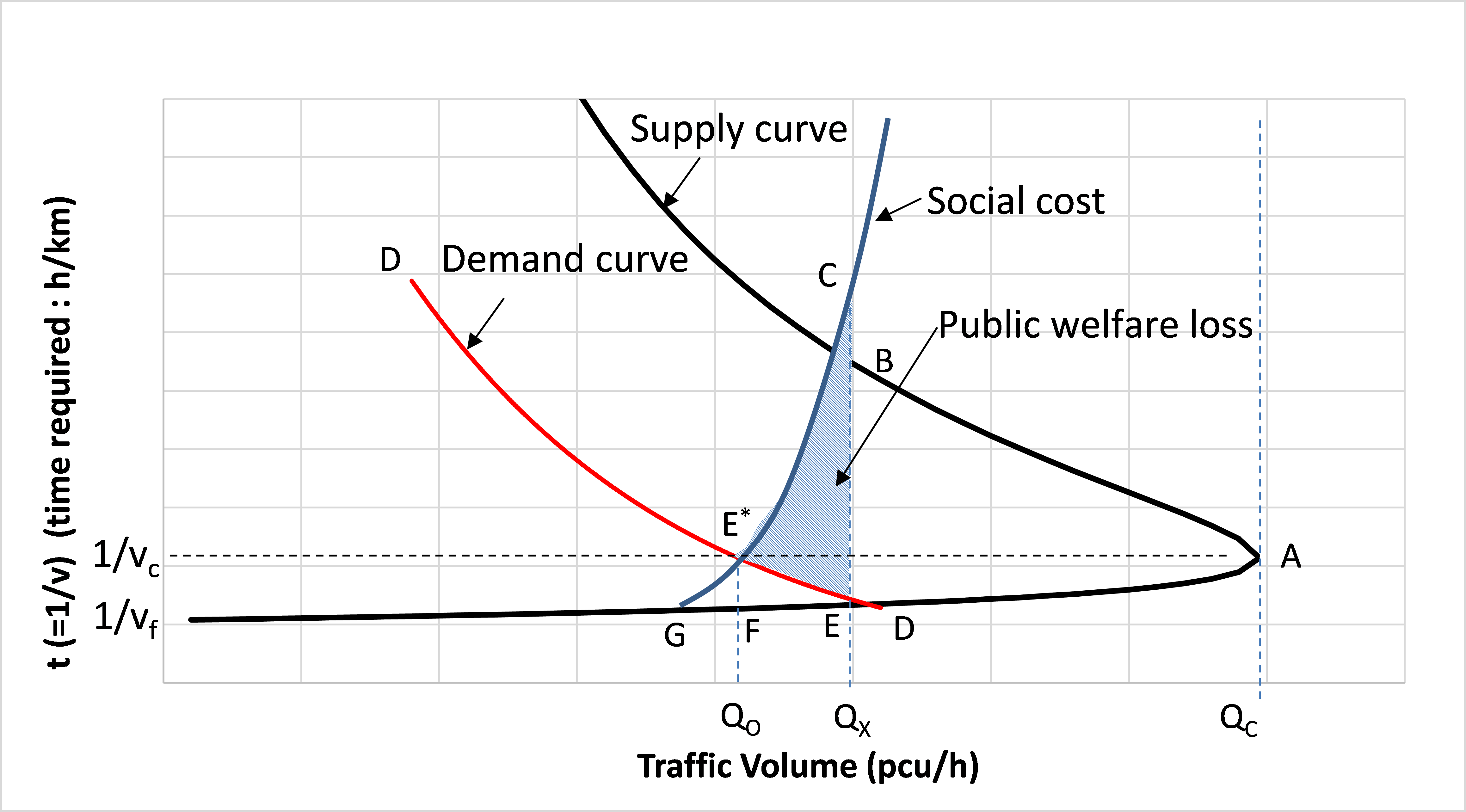Figure 8: Road Traffic Service Market

In Figure 8, the point A is called hyper congestion condition at critical traffic volume (q_c) when traffic volume becomes larger beyond point A, travel time takes longer because of traffic congestion. There are two travel time (t) except point A. For instance, there are point E and point B at a certain traffic volume (Q_x). In case of point B, the travel time takes longer than that of at point E. If traffic demand curve D-D is given, the point E is cross point between demand curve D-D and supply curve which provides balance condition between traffic demand and supply. If social cost curve is given, the point E* becomes balance point between traffic demand and social cost. Then area CE*E provides traffic service cost loss caused by traffic congestion because infrastructure should cover at the level of traffic volume (Q_x) at the point E and social cost rises at the point C where its traffic volume (Q_x) is same as that of at the point E. Therefore area CE*E is defined as the public welfare loss which means traffic congestion social loss.

In order to calculate the public welfare loss from measurement data, it is necessary to define condition for each curve of Figure 8 from the actual measurement analyzed data.  The condition of traffic congestion social loss is as follows:

• Supply curve is q– v curve form envelopment observation.
• The critical speed (v_c) is used at SR=0.65 because this point is congestion threshold.
• Demand curve D-D is used from actual measurement traffic data.
• The social cost curve is unknown under this condition. Therefore BE* liner curve is taken.
• The congestion social loss is defined as area BE*E instead of area CE*E.

The Figure 9 shows the congestion social loss calculation example at Camera#2 with this quantitative social loss analysis. The result of Social loss analysis at all locations shows in Table 1. According Table 1, it is clear relationship between Speed Ratio (SR) and Social loss value.

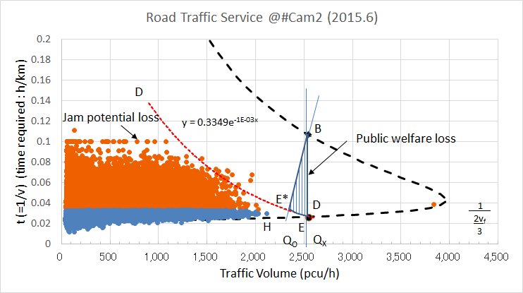Figure 9: Road Traffic Service Market at Camera#2

Table 1: Social Loss and Speed Ratio

Location	SR(vave/vf)	Social Loss
Camera#1	0.66	3.3
Camera#2	0.57	8.1
Camera#3	0.66	3.1
Camera#4	0.69	3.2
Camera#5	0.69	2.0
Camera#6	0.63	2.2
Camera#7	0.69	1.3
Camera#8	0.73	0.2
Camera#9	0.69	1.6
Camera#10	0.67	2.4
VMS#3	0.72	0.7

3. Traffic Congestion Analysis

In the previous section, the envelopment observation method is used for getting traffic flow equation from its measurement. Based on the each traffic flow equation, new quantitative social loss of traffic congestion analysis is introduced. In terms of traffic congestion judgement, the average vehicle speed is used. This average vehicle speed is different at each road and its condition. Therefore it is necessary to have some relative vehicle speed compared with normal driving speed which is taken as free speed in this paper. As for traffic congestion judgement, the average speed is not only parameter but also the traffic occupancy for example.

3.1.  Traffic Occupancy

The traffic occupancy is used for one of parameters which shows the level of traffic congestion condition. There are two traffic occupancies in the theory, time occupancy and space occupancy. In real traffic management, time occupancy is often used for the freeway [7]. In this section, time occupancy is used. The time occupancy is defined the percentage ratio between total measurement time (t) of the vehicles to a certain block of road section under certain time frame. The formula of time occupancy is provided by (5).

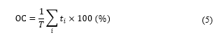where T is time of measurement, (t_i) is detected time of vehicle (i )[8].

When number of existing vehicle a certain section is (N), average length of vehicle is (  ) in (6) is given.

Therefore occupancy (OC) is proportional to traffic density (k) and traffic volume (q).

From the one month measurement data of Camera#1 and #2 in June 2015, traffic density (k) to occupancy (OC) relationship are shown in Figure 10. According to Figure 10, the relationship between (k) and (OC) is proportional.

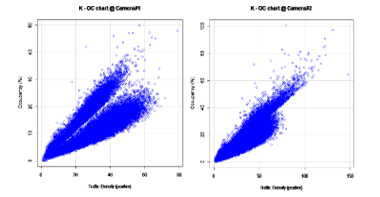Figure 10: Example of k – q curve at Camera#1 and Camera#2

From Figure 10, it seems that the measurement data is plotted into two groups. In the section 3.3, time zone analysis is introduced because traffic congestion is dependent with time of a day (refer to Figure 6) [9].

3.2.  Daily Traffic Condition

In this section, a daily traffic changes of traffic volume and velocity is described. In Figure 11, there are two cases of daily based traffic condition at Camera#1 and #2. The graph shows one month traffic volume changes from 7:00 am to next day 6:00 am and average vehicle velocity changes. There are two peaks of traffic volume in each case. One peak occurs between 7:00 am to 10:00 am and the second peak occurs between 18:00 to 20:00. When vehicle average speed is concerned, there is not so much changes of velocity in Camera#1 but different speed at Camera#2. In case of Camera#2, there is a drop during the second peak volume of traffic. And each graph shows classification by four cases—total one month average, weekday, Saturday, and Sunday. According to Figure 11, there is traffic jam in Camera#2 between 18:00 to 20:00 and the average vehicle speed goes down to less than 20 km/h which is confirmed the speed under heavy traffic congestion through the recorded traffic monitoring video data.

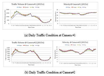Figure 11: Daily Traffic Condition at Camera#1 and Camera #2

3.3.  Occupancy and Traffic Density

As described in section 3.1, time zoning is adapted into  Figure 10. In this section,  six time zone is defined as shown in Table 2

Table 2: Social Loss and Speed Ratio

Zone Name	Time Zone
T1	7:00 ―  10:59
T2	11:00 ―  14:59
T3	15:00 ― 18:59
T4	19:00 ― 22:59
T5	23:00 ― 2:59
T6	3:00 ― 6:59

There are 6 time zones such as T1 is defined time frame from 7:00 am to 10:59 am which is most congested time frame as we see in Figure 11. And T4 is defined time frame from 19:00 to 22:59 which is the second congested time frame. In case of using this Time Zone classification for k – OC curve, Time Zone based k – OC curve is shown in Figure 12. In this paper, we focus on the characteristics at Camera#1 and #2.

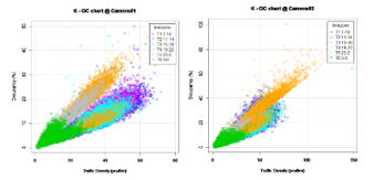Figure 12: Time Zone based k – OC curve at Camera#1 and Camera#2

When the Time Zone based analysis, it is clear two groups data plot in Camera#1, where there is no traffic congestion condition compared with that of Camera#2. From the result of Camera#1 analysis, the upper group in k – OC curve comes from majority of T4 (19:00-22:59). The lower group in k –OC curve comes from T1, T2, and T3. In another words, upper part of T4 is relative lower density compared with lower part of T4. This means there are two types of traffic congestion condition. Therefore one type of traffic congestion is defined as low density traffic congestion (herein after it is called as Low density Congestion) and the other one is higher traffic density congestion (herein after it is called as High density Congestion).

The next section describes traffic volume to occupancy and average vehicle speed to occupancy in order to understand the traffic congestion condition with other traffic parameters.

3.4.  Occupancy and Traffic Volume and Speed

In Figure 11, it is shown about the daily traffic condition by traffic volume and average vehicle speed. In this section, it adapts Time Zone basis analysis for q–OC curve and v–OC curve in order to understand relationship between traffic volume to occupancy and  average vehicle speed to occupancy.

The Traffic volume (q) to Occupancy (OC) Time Zone basis relationship at Camera#1 and #2is shown in Figure 13.

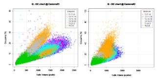Figure 13: Time Zone based q – OC curve at Camera#1 and Camera#2

From the q – OC curve at Camera#1 in Figure 13, it shows more clear about difference between Low density congestion area and High density congestion area. The Low density congestion occurs in T4.  It looks same trend of characteristics at Camera#2 but there is no clear two groups separation between Low density congestion and High density congestion.

The next Figure 14 shows average vehicle speed (v) to Occupancy (OC) relationship.

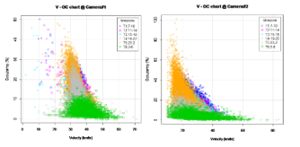Figure 14: Time Zone based v – OC curve at Camera#1 and Camera#2

From Figure 14, it is clear that traffic congestion at lower than 30km/h occurs above 30% Occupancy condition.

Here is a question why Low density congestion occurs. It is considered at the next discussion section.

4. Discussion of Low density congestion

According to all traffic measurement location in Ahmedabad, the location Camera#2 is the most congested condition location (refer to Figure 5). And traffic condition during T4 time zone becomes most congested as described in previous section. The traffic volume at T4 of Camera#2 is the second peak of traffic volume in a daily condition as shown in Figure 6 (b) and Figure 11 (b). The highest peak of traffic volume occurs at  T1 and T2. Therefore it is possible to define that High density congestion occurs at T1 and T2 and Low density congestion occurs at T4.

There is one more traffic parameter which is called Headway. The Headway is defined the distance between the front of driving vehicle group and the front of the second driving vehicle group (refer to Figure 15).

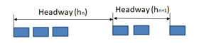Figure 15: Headway definition

It is relative true the relationship between the small value of Headway and traffic congestion because its traffic density is large. The Headway ( ) and the traffic density relationship is described (7) from the theory.

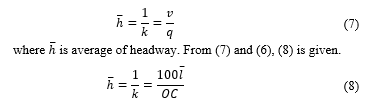From (8), the headway ( ) is inverse proportional to occupancy (OC) with the average of vehicle length ( ). The average of vehicle length is difficult to get from real measurement. Therefore the relationship between the average headway ( ) to occupancy (OC) is not exactly inverse relation. The Figure 16 shows  – OC curve at Camera#1 and #2. The vertical axis is legalism for clear display.

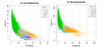Figure 16: Time Zone based

From Figure 16, the traffic congestion occurs at T4 Time Zone and its Occupancy is above 30%.  In this analysis, it is difficult to clarify between Low density congestion and High density congestion. The difference of Low density congestion and High density congestion becomes clear from traffic volume to occupancy or traffic density to occupancy relationship.

When it check the Time Zone of Low density, T4 and time period is from 18:00 to 22:59. After discussion with local traffic police, they observe that the Low density congestion may be  caused by limitation of parking space in the city. In the evening after work, the residents of Ahmedabad stop by restaurants and or shopping place and they make parking their vehicle at not permitted place such as along the street. Therefore this parking issues have potential for creating Low density congestion. If so, there is a solution for Low density congestion by preparing appropriate parking space for restaurant and shopping. The reason why the Low density congestion is detected by the traffic monitoring cameras is assumed that the collecting data is based on number of driving vehicles, not parking vehicles. For the traffic monitoring cameras, they take the vehicles as a part of side roads, which means parking vehicles make roads just narrow path and is unable to count the vehicles number as their traffic density. This situation tells that it is important to judge the traffic monitoring data by not only numerical data from the monitoring camera but also actual visual data.

In terms of quantitative social loss analysis method, the demand curve in Figure 9 is used from the measurement data, which is described as the condition of the quantitative social loss analysis method. When Figure 9 is mapped by time zone, it becomes Figure 17.

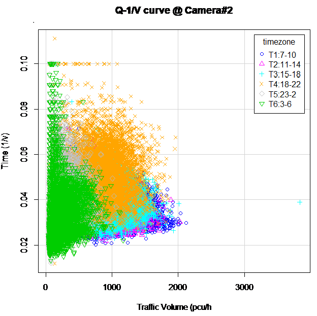Figure 17: Time Zone based q-1/v curve at Camera#2

From Figure 17, Low density congestion area at T4 is located inside the demand curve. Therefore it is able to confirm proposed quantitative social loss analysis is valid.

5. Summary

In this study, there are three features for Indian traffic flow analysis.

• Feature 1: Introduce envelop observation method based on traffic flow data to provide traffic flow fundamental characteristics by traffic flow equation. It is able to get traffic flow parameters from this equation i.e. jam density (k_j), free speed (v_f).
• Feature 2: Propose quantitative social loss of traffic congestion method by only using traffic measurement data. As for critical speed (v_c), it is defined by Speed Ratio (SR)―average speed (v_ave) to free speed (v_f)―65 or 2/3 of (v_f), which is based on traffic flow analysis in India.
• Feature 3: There are two types traffic congestion condition in India, Low density congestion and High density congestion. It is presumed that Low density congestion mainly is caused by parking vehicle problem. Therefor Indian Traffic congestion occurs not only by large number of vehicles but also other infrastructure issues.

All this study analysis is based on one month of real traffic flow data in Ahmedabad city. It is necessary to have more different timing, location i.e. place, city, country. It is also important to have traffic video data in order to evaluate traffic congestion condition and understand congestion reason. The above all research items are future work.

Conflict of Interest

There is no conflict of interest in this study.

Acknowledgment

This study also underwent the program ID:JPMJSA1606 of the International Science and Technology Cooperation Program (SATREPS) challenges for global challenges in 2016.

Special appreciation to Mr. Kikuchi.C and Mr. Mallesh.B of Zero-Sum ITS India for providing traffic data in Ahmedabad.

1.  A. Tandiya, S. Akthar, M. Moussa, and C. Tarray, “Automotive semi-specular surface defect detection system,” in 2018 15th Conference on Computer and Robot Vision (CRV), May 2018, 285-291. DOI: 10.1109/CRV.2018.00047
2.  C. Fernandez, C. Platero, P. Campoy, and R. Aracil, “Vision system for on-line surface inspection in aluminum casting process,” in Proceedings of IECON ’93 – 19th Annual Conf. of IEEE Industrial Electronics, 15-19 Nov. 1993, 1854 – 1859. DOI: 10.1109/IECON.1993.339356
3.  Z. Liu, W. Wang, X. Zhang, and W. Jia, “Inspection of rail surface defects based on image processing,” CAR 2010 – 2010 2nd Int. Asia Conf. Informatics Control. Autom. Robot., vol. 1, pp. 472-475, 2010. DOI: 10.1109/CAR.2010.5456793
4.  Y.-G. Cen, R.-Z. Zhao, L.-H. Cen, L. Cui, Z. Miao, and Z. Wei, “Defect inspection for TFT-LCD images based on the lowrank matrix reconstruction,” Neurocomputing, vol. 149, 1206- 1215, 2015. DOI:10.1016/j.neucom.2014.09.007
5.  B. Liu, S. Wu, and S. Zou, “Automatic detection technology of surface defects on plastic products based on machine vision,” 2010 International Conf. on Mechanic Automation and Control Engineering, MACE2010, 2213 – 2216, 07 2010. DOI: 10.1109/MACE.2010.5536470
6. J. Guo and W. Shao, “Automated detection of surface defects on sphere parts using laser and CDD measurements,” IECON 2011 – 37th Annu. Conf. IEEE Ind. Electron. Soc., pp. 2666-2671, 2011. DOI: 10.1109/IECON.2011.6119732
7.  S. Janardhana, J. Jaya, K. J. Sabareesaan, and J. George, “Computer aided inspection system for food products using machine vision A review,” 2013 Int. Conf. Curr. Trends Eng. Technol., pp. 29 – 33, 2013. DOI: 10.1109/ICCTET.2013.6675906
8. P. M. Cho CS, Chung BM, “Development of real-time vision based fabric inspection system,” IEEE Trans. Ind. Electronics, vol. 52(4), 1073–9, 2005.
9.  S. V. der Jeught and J. J. Dirckx, “Real-time structured light profilometry: a review,” Optics and Lasers in Engineering, vol. 87, 18 – 31, 2016, Digital optical & Imaging methods in structural mechanics. https://doi.org/10.1016/j.optlaseng.2016.01.011
10.  D. Palouek, M. Omasta, D. Koutny, J. Bednar, T. Kouteck,and F. Dokoupil, “Effect of matte coating on 3D optical measurement accuracy,” Optical Materials, vol. 40, 02 2015. https://doi.org/10.1016/j.optmat.2014.11.020
11.  M. C. Knauer, J. Kaminski, and G. Hausler, “Phase measuring deflectometry: a new approach to measure specular free-form surfaces,” in Optical Metrology in Production Engineering, ser. procspie, W. Osten and M. Takeda, Eds., vol. 5457, 366-376, Sep. 2004. https://doi.org/10.1117/12.545704
12.  I. G. O. Kafri, “Moire deflectometry: A ray deflection approach to optical testing,” Optical Engineering, vol. 24, no. 6, 944 -960, 1985. [Online]. Available: https://doi.org/10.1117/12.7973607
13.  M. Servn, R. Rodriguez-Vera, M. Carpio, and A. Morales, “Automatic fringe detection algorithm used for Moire deflectometry,”Applied optics, vol. 29, 3266 – 70, 08 1990.
14.  B. Wang, X. Luo, T. Pfeifer, and H. Mischo, “Moire deflectometry based on Fourier-transform analysis,” Measurement,vol. 25, 24 – 253, 06 1999. https://doi.org/10.1016/ S0263-2241(99)00009-3
15.  A. E.-R. Ricardo Legarda-Senz, “Wavefront reconstruction using multiple directional derivatives and Fourier transform,” Optical Engineering, vol. 50, no. 4, 1 – 4 , 2011. [Online]. Available: https://doi.org/10.1117/1.3560540
16. D. Fontani, F. Francini, D. Jafrancesco, L. Mercatelli, and P. Sansoni, “Mirror shape detection by ”Reflection Grating Moire Method” with optical design validation,” Proceedings of SPIE – The International Society for Optical Engineering 5856, Jun 2005. DOI: 10.1117/12.612114
17.  S.-W. K. Ho-Jae Lee, “Precision profile measurement of aspheric surfaces by improved Ronchi test,” Optical Engineering, vol. 38, no. 6, 1041 – 1047, 1999. [Online]. Available:https://doi.org/10.1117/1.602147
18.  G. P. Butel, G. A. Smith, and J. H. Burge, “Binary pattern deflectometry,” Appl. Opt., vol. 53, no. 5, 923 – 930, Feb 2014. [Online]. Available: http://ao.osa.org/abstract. cfm?URI=ao-53-5-923
19.  J. L. H. Willem D. van Amstel, Stefan M. B. Baumer, “Optical figure testing by scanning deflectometry,” Proc. SPIE 3739, Optical Fabrication and Testing, 6 September 1999. doi: 10.1117/12.360155, Available: https://doi.org/10.1117/ 12.369201
20.  S. Krey, W. D. van Amstel, K. Szwedowicz, J. Campos, A. Moreno, and E. J. Lous, “Fast optical scanning deflectometer for measuring the topography of large silicon wafers,” Proc. SPIE 5523, Current Developments in Lens Design and Optical Engineering V, 14 October 2004. doi: 10.1117/12.559702, https://doi.org/10.1117/12.559702
21.  K. Ishikawa, T. Takamura, M. Xiao, S. Takahashi, and K. Takamasu, “Profile measurement of aspheric surfaces using scanning deflectometry and rotating autocollimator with wide measuring range,” Measurement Science and Technolog, vol. 25, no. 6, Apr 2014. [Online]. Available: https://doi. org/10.1088%2F0957-0233%2F25%2F6%2F064008
22.  Y. Tang, X. Su, Y. Liu, and H. Jing, “3D shape measurement of the aspheric mirror by advanced phase measuring deflectometry,” Opt. Express, vol. 16, no. 19, 15090 – 15096, Sep 2008. [Online]. Available: http://www.opticsexpress.org/ abstract.cfm?URI=oe-16-19-15090
23.  D. Malacara, Optical Shop Testing (Wiley Series in Pure and Applied Optics), Wiley-Interscience, 2007.
24.  A. V. Maldonado, P. Su, and J. H. Burge, “Development of a portable deflectometry system for high spatial resolution surface measurements,” Appl. Opt., vol. 53, no. 18, 4023 – 4032, Jun 2014. https://doi.org/10.1364/AO.53.004023
25.  C. Horneber, M. Knauer, and G. Husler, “Phase measuring deflectometry – a new method to measure reflecting surfaces,” Annual Report Optik, 01 2000.
26.  J. Xiao, X.Wei, Z. Lu,W. Yu, and H.Wu, “A review of available methods for surface shape measurement of solar concentrator in solar thermal power applications,” Renewable and Sustainable Energy Reviews, vol. 16, no. 5, 2539 – 2544, 2012. https://doi.org/10.1016/j.rser.2012.01.063
27.  C. E. Andraka, S. Sadlon, B. Myer, K. Trapeznikov, and C. Liebner, “Rapid reflective facet characterization using fringe reflection techniques,” Proceedings of the Energy Sustainability, 19 – 23, 2009. DOI: 10.1115/1.4024250
28.  C. Devivier, F. Pierron, and M. Wisnom, “Damage detection in composite materials using deflectometry, a full-field slope measurement technique,” Composites Part A: Applied Science and Manufacturing, vol. 43, no. 10, 1650 – 1666, 2012. https://doi.org/10.1016/j.compositesa.2011.11.009
29.  J. Geng, “Structured-light 3D surface imaging: a tutorial,” Adv. Opt. Photon., vol. 3, no. 2, 128–160, Jun 2011. https: //doi.org/10.1364/AOP.3.000128
30.  M. Kujawinska and J. Wjciak, “High accuracy Fourier transform fringe pattern analysis,” Optics and Lasers in Engineering,vol. 14, no. 4, 325 – 339, 1991. https://doi.org/10.1016/0143-8166(91)90056-Y
31.  M. Takeda, H. Ina, and S. Kobayashi, “Fourier-transform method of fringe-pattern analysis for computer-based topography and interferometry,” J. Opt. Soc. Am., vol. 72, no. 1, 156- 160, Jan 1982. https://doi.org/10.1364/JOSA.72.000156
32.  L. Armesto, J. Tornero, A. Herraez, and J. Asensio, “Inspection system based on artificial vision for paint defects detection on cars bodies,” in Robotics and Automation (ICRA), 2011 IEEE International Conference on, 1–4, 9-13 May 2011. DOI: 10.1109/ICRA.2011.5980570
33.  C. Tarry, M. Stachowsky, and M. Moussa, “Robust detection of paint defects in moulded plastic parts,” Proc. – Conf. Comput. Robot Vision, CRV 2014, 306–312, 2014. DOI: 10.1109/CRV.2014.48
34.  T. Liu, C. Zhou, Y. Liu, S. Si, and Z. Lei, “Deflectometry for phase retrieval using a composite fringe,” Optica Applicata, vol. 44, no. 3, 451 – 461, 2014. DOI: 10.5277/oa140309
35.  Y. Surrel, “Deflectometry: A simple and efficient noninterferometric method for slope measurement,” Xth SEM Int. Congr. Exp. Mech., 2004.
36.  K. Hibino, B. F. Oreb, D. I. Farrant, and K. G. Larkin, “Phase shifting for nonsinusoidal waveforms with phase-shift errors,” J. Opt. Soc. Am. A, vol. 12, no. 4, p. 761, 1995. https: //doi.org/10.1364/JOSAA.12.000761
37.  E. Stoykova, J. Harizanova, and V. Sainov, “Pattern Projection Profilometry for 3D Coordinates Measurement of Dynamic Scenes,” Three-Dimensional Telev., pp. 85–164, 2008. DOI: 10.1007/978-3-540-72532-9_5

(Click Here)

(Click Here)