1. Introduction

Big data refers to an extremely large volume of information, whose analysis cannot be done in real-time using standard techniques. Analyzing big data includes, but is not limited to, extracting useful information for a particular application and determining possible correlations among various samples of data. Major challenges of big data are enormous sample sizes, high dimensionality problems, and scalability limitations of technologies to process the growing amount of data [1]. Knowing these challenges, researchers are seeking various methods to analyze Big Data through several approaches like different machine learning and computationally intelligent algorithms.

Machine learning (ML) algorithms and computationally intelligent (CI) approaches plays a significant role to analyze big data. Machine learning has the ability to learn from the big data and perform statistical analysis to provide data-driven insights, discover hidden patterns, make decisions and predictions [2]. On the other hand, the computational intelligence approach enables the analytic agent/machine to computationally process and evaluate the big data in an intelligent way [3] so, big data can be utilized efficiently. Particularly, one of the most crucial challenges of analyzing big data using computational intelligence is searching through a vast volume of data, which is not only heterogeneous in structure but also carries complex inter-data relationships. Machine learning and computational intelligence approaches help in big data analysis by providing a meaningful solution for cost reduction, forecasting business trends and helps in feasible decision making considering reasonable time and resources.

One of the major challenges of machine learning and computational intelligence is an effective feature extraction approach, which is a difficult combinatorial optimization problem [4]. A feature is a measurable property, which helps to determine a particular object. The classification accuracy of a machine learning method is influenced by the quality of the features extracted for learning from the dataset. Correlation between features [5] carries great influence on the classification accuracy and other performance measures. In a large dataset, there may be a large number of features which do not have any effect or may carry a high level of interdependence that may require advanced information theoretic models for meaningful analysis. Selecting proper and reasonable features from big data for a particular application domain (such as cyber security, health and marketing) is a difficult challenge and if done correctly, could play a significant role in reducing the complexity of data.

In the domain of combinatorial optimization, selecting a good feature set is at the core of machine learning challenges. Searching is one of the fundamental concepts [6] and is directly related to the famous computation complexity problems such as Big-O notations and cyclomatic complexity. Primarily, any problem that is considered a searching problem looks for finding the “right solution,” which is translated in the domain of machine learning as finding a better local optimum in the search space of the problem. Exhaustive search [7] is one of the methods for finding an optimal subset of the solution, however, performing an exhaustive search is impractical in real life and will take a huge amount of time and computational resources for finding an optimal subset of the feature set to provide a solution.

In a combinatorial optimization problem, there is a finite or limited number of solutions available in the solution space. Most of the combinatorial optimization problems are considered as a complicated problem [8]. Simulated Annealing (SA) is one of the computational intelligence approaches for providing meaningful and reasonable solutions for combinatorial optimization problems [9] [10] and can be utilized for feature extraction (example; for cybersecurity threat detection). As per our literature survey, it is found that simulated annealing is usually not utilized as a classifier [11]. However, the SA method is explored a lot for searching optimal solutions to problems such as the travelling salesperson problem [12], color mapping problem [8], traffic routing management problem [13], and clustering of large sets of time series [14].

State of the art research in merging ML and CI algorithms has demonstrated promise for different applications such as electricity load forecasting [15], pattern classification [16], stereovision matching [17]  and most recently for feature selection [18]. In a practical application, it is required to find a reasonably better feature set that can be utilized for cyber intrusion detection with relatively better reliability and performance. This paper addresses this challenge empirically using various datasets and proposes a methodological approach.

In this paper, we have introduced an intelligent computational approach merging Simulated Annealing (SA) and Support Vector Machine (SVM) with an aim to provide a reasonable solution for extracting optimum (minimum) features from a finite number of features. The classifier is designed with the goal of maximizing the detection performance measures, and the combinatorial optimizer is designed to determine an optimal feature subset, which is input to the classifier. We have applied this general methodology on two different Network intrusion datasets; UNSW dataset (Australian Centre for Cyber Security) [19] [20] and UNB dataset (Canadian Institute of Cyber Security) [21] in order to analyze the performance of the proposed method and evaluate whether the outcome can provide an optimum feature subset and can detect the presence of intrusion in the network system. Furthermore, the empirically validated outcomes of the proposed method are evaluated in contrast with other machine learning methods like general SVM (without annealing) and decision tree to analyze which methodology provides a better reasonable solution.

2. Background Research

Various research works have been conducted to find an effective and efficient solution for combinatorial optimization problems (optimum feature subset selection) for network intrusion detection to ensure network security and for various other applications. An ideal intrusion detection system should provide good detection accuracy and precision, low false positive and negative, and better F1-score. However, nowadays for the increasing number of intrusions, software vulnerabilities raise several concerns to the security of the network system. Intrusions are easy to launch in a computing system, but it is challenging to distinguish them from the usual network behavior. A classifier (that classifies normal and anomalous behavior) is designed with the goal of maximizing the detection accuracy and the feature subset utilized by the classifier is selected as the optimal feature subset. Researchers have been trying to develop different solutions for different types of scenarios. Finding an optimum feature subset for reliable detection system is a significant combinatorial optimization problem in network intrusion detection. Some of the related works are described below based on the approaches in different sectors (cybersecurity, electricity bill forecasting, tuning SVM kernel parameters) and advantages and disadvantages.

In [22], the authors proposed a combined SVM based feature selection model for combinatorial optimization problem in which they applied convex function programming additionally to the general SVM programming to find an optimal subset of features. This approach consumes more computational resources, and the process is mathematically complex.

In [23-25], the authors provided a signature-based detection method which is capable of detecting DoS and routing attack over the network. In [24] the authors mentioned a signature-based model such that the total network system is divided into different regions, and to build a backbone of the monitoring nodes per region they established a hybrid placement philosophy [26]. However, this method was limited to the known signature models.  If the signature is not updated and unknown to the nodes at the different region, it does not find a match, and the intrusion walks inside the system. In this proposed system, there were no approaches to finding an optimal feature set to determine any unknown type attacks.

In [27], the authors also proposed a signature-based model in which each of the nodes will verify packet payload and the algorithm will also skip a large number of unnecessary matching operation resulting low computational costing and comparison differentiate between standard payloads and attacks [26]. This is a fast process of identifying malicious activity but when the complexity of the signatures increases it may be unable to detect the malicious packet.

In [28], the authors proposed an OSVM (Optimized Support Vector Machine) based detection approach in which the outliers are rejected and make it easier for the algorithm to classify attacks with precision. For more massive datasets which have some feature dimension then this algorithm does not perform well as it does not know which features to use as the feature workspace is very high, resulting the algorithm performing an exhaustive search on the whole workspace. The proposed method does not provide any reasonable solution for the optimum feature extraction method.

In [29], the authors proposed a random forest-based intrusion detection mechanism that was applied to both anomaly and signature-based data samples. The random forest-based approach works fine on the signature-based approach, but the algorithm was unable to detect malicious characteristic with an excellent detection accuracy. Also, when applied on large dataset the complexity of detection was very high for this algorithm to perform.

In [30], the authors proposed decision tree-based wrapper intrusion detection approach in which the algorithm can detect a subset of the feature among all the features available on the KDD dataset. So it reduced the computational complexity of the classifier and provided high accuracy of detection intrusion. However, it also performs an exhaustive search trying all possible feature subsets to provide an output. If the feature numbers are high, also data set is large then doesn’t provide good accuracy regarding detection accuracy and consumes much time. In real time scenario, this method may fail to detect an anomaly within the secured time limit.

In [31], the authors introduced a lightweight intrusion detection methodology in which energy consumption is considered as a detection feature to detect abnormal behaviors on the network flow. When the energy consumption diverges from an anticipated value, the proposed method calculates the differences of the values, and the algorithm classifies the anomaly from the normal behavior. They minimized the computational resources by focusing only on the energy consumption, so algorithm works faster and provides an acceptable solution for the intrusion detection. In anomaly-based detection scheme as the characteristic behaviors of the data packets are analyzed, what if the node does not consume more energy it consumes more than the specified time to transfer data over to the network? It may be compromised by modification attack which creates a time delay in the route from source to destination. This algorithm becomes vulnerable if the characteristic of the anomaly is different rather than energy consumption. A single feature is not sufficient enough to detect a particular attack precisely.

In [31], the authors proposed in their research on intrusion detection that network nodes must be capable of detecting even small variations in their neighborhood and the data has to be sent to the centralized system. They proposed three algorithms on the data sent by the node to find such type of anomaly namely wormhole. They claimed that their proposed system is suitable for IoT as it consumes low energy and memory to operate [23]. However, analyzing the data samples using three types of algorithm consumes a massive amount of time and limits the countermeasure effectiveness of the algorithm as its huge taking time to detect attacks in real time scenario. Also when the network facing huge traffic flow the algorithm may not be detecting intrusion in the secured time limit.

In [32], the authors proposed a group-based intrusion detection system, which uses a statistical method and designed a hierarchical architecture-based system. The results were very highlighting as their detection accuracy was very high, low false alarm rate, low transmission power consumption. However, the method does not seem feasible if multiple features are considered and don’t provide any information about the process of selecting multiple features. Thus, the combinatorial optimization exists in such a scenario.

In [33], the authors used artificial intelligence artificial neural network scheme where ANN is used to every sensor node. The algorithm provides self-learning ability to the intrusion detection system. ANN is an excellent approach in intrusion detection, but node energy consumption becomes high as its continuously learning from the data packet flow.

In [34], the authors proposed an efficient impostor alert system against sinkhole attacks. In this system, a record of the suspected network nodes is generated by continuously analyzing the data. After that, the data flow information’s are used to identify the intrusion in the system. When traffic volume is high, and a lot of data packets are flowing, there may be a scenario that many nodes are in the suspect list and comparing all of them may limit the network performances. The algorithm in this research is performing an exhaustive search for finding an optimal feature subset for sinkhole attack detection.

In [29], the authors proposed a random forest-based intrusion detection mechanism that was applied to both anomaly and signature-based data samples. The random forest-based approach works fine on the signature-based approach, but the algorithm was unable to detect malicious characteristic with an excellent detection accuracy. Also, when applied on large dataset the complexity of detection was very high for this algorithm to perform.

In [30], the authors proposed decision tree-based wrapper intrusion detection approach in which the algorithm can detect a subset of the feature among all the features available on the KDD dataset. So, it reduced the computational complexity of the classifier and provided high accuracy of detection intrusion. However, it also performs an exhaustive search trying all possible feature subsets to provide an output. If the feature numbers are high, also data set is large then doesn’t provide good accuracy regarding detection accuracy and consumes much time. In real time scenario, this method may fail to detect an anomaly within the secured time limit.

3. Background of Machine Learning Algorithm

3.1.  Support Vector Machine

The Support vector machine (SVM) [35] is a discriminative and normally supervised machine learning methodology that analyzes training samples to process a wide variety of classification problems. The algorithm generates an optimal hyperplane which classifies training examples and new data samples. This supervised learning method can analyze the data samples to perform handwritten character recognition [36], face detection [37], pedestrian detection [38], text categorization.

Consider a training dataset , where   represents the training examples with  dimensional input features, p is the number of training examples, and  represents the desired or labelled output of the  training data sample.  denotes output of the  positive training samples and denotes the output of the  negative training samples.

Based on the above consideration, the decision hyperplane is given by (1).

The  and  represent the weight vector and bias term, respectively. During the training process, the weight and the bias terms are learned. With these learned parameters, the decision hyperplane places itself at an optimum location between the positive and negative training example clouds. SVM places the decision boundary in such a way that it maximizes the geometric margin of all the training data samples. In other words, all training examples have the greatest possible geometric distance from the decision boundary.  The optimization problem is given by (2).

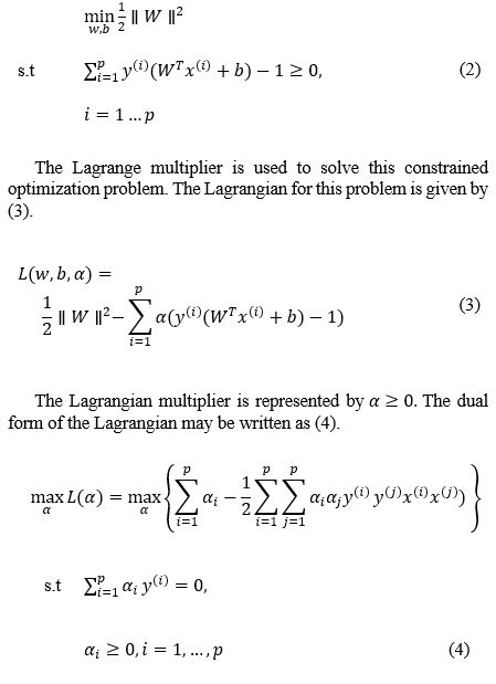
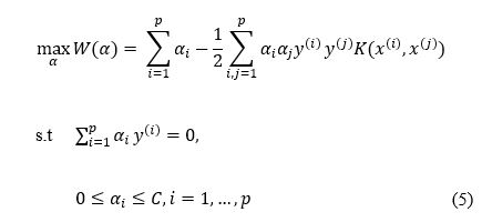
The solution above drives the optimum decision surface that can distinguish linearly separable positive and negative training data example clouds. However, for non-linearly separable training data, a suitable kernel and regularization may be applied. The Gaussian kernel is widely used in such types of problems. Applying a kernel and regularization to (4) gives (5) (C is the regularization parameter).

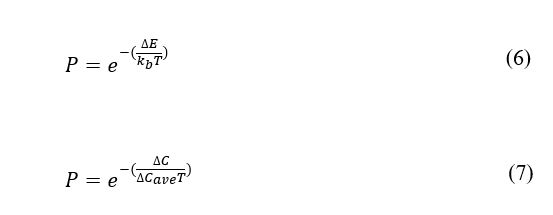
Simulated Annealing can be described as an iterative procedure that is composed of two loops. The outer loop is known as a cooling loop and the inner loop as a thermal equilibrium loop. The algorithm is initialized by several parameters like the number of cooling loops, number of equilibrium loops, and probability function. The purpose of the inner loop is to find the best solution for the given temperature to attain thermal equilibrium at the given temperature state. In each equilibrium loop, the algorithm takes a small random perturbation to create a new candidate solution. Initially, as the algorithm does not know which direction to search, it picks a random direction to search, and an initial solution is created. A cost function determines the goodness of the solution. A small random perturbation is made to the current solution because it is assumed that good solutions are generally close to each other, but it is not guaranteed as the best optimal solution. Sometimes the newly generated solution results in a better solution, then the algorithm keeps the new candidate solution. If the newly generated solution is worse than the current solution, then the algorithm decides whether to keep or discard the worse solution, which depends on the evaluation of Boltzmann’s probability function, which is given by          (6).

3.2.  Simulated Annealing

The change in energy ∆E can be estimated by the change in the cost function ∆C, corresponding to the difference between the previously found best solution at its temperature state and the cost of new candidate solution at the current state. Boltzmann’s constant may be estimated by using the average change in cost function ( . Thus, Boltzmann’s function may be estimated using        (7).

After running the inner loop for the prescribed number of times, wherein each loop it takes a new better solution or keeps a worse solution, the algorithm may be viewed as taking a random walk in the solution space to find a sub-optimal solution for the given temperature.

The current best solution will be recorded as the optimal solution. The temperature is decreased according to a basic linear decrease schedule. The initial temperature is set to a very high value initially, because it allows the algorithm to explore a wide range of solutions, initially. The final temperature should be set to a low value that prevents the algorithm to accept a worse solution at the last stages of the process. If the number of the outer loops has not reached zero, then the inner loop is called again otherwise the algorithm terminates.

3.3.  Decision Trees

Decision tree [39] is a machine learning mechanism which is mostly used for classification and regression in many application domains. Decision trees are based on conceptual tree analytical model that considers dependency perception of an object in such a way that the branches of the tree represent the dependency, and the leaf of the tree represents the object itself regarding the classification labels (such as logical 0 or logical 1) [40]. Further, research literature shows that decision trees are used to represent the extraction of dependent features from a data set where the branches represent the feature or attribute while the leaf represents the decision using class labels. Decision trees are mostly used in data mining and machine-learning research works [41].

There are several decision tree algorithms such as ID3 [42], C4.5 (improved from ID3) [43] and CART (Classification and Regression Tree) [44]. CART based decision tree algorithm is used mainly for machine classification purposes [45].

CART [46] can be used for classification of categorical data or regression of continuous data. CART algorithm is designed to develop trees based on the sequence of rules. If the object passes a specific rule, it goes into one structure otherwise it is sent to other structure. Further, the rules or questions defines the next step to follow. For example, there are two random variables and . Let’s say there are decision thresholds or rules are  and . If < , go and check if <  otherwise, go and check if <  and so on.

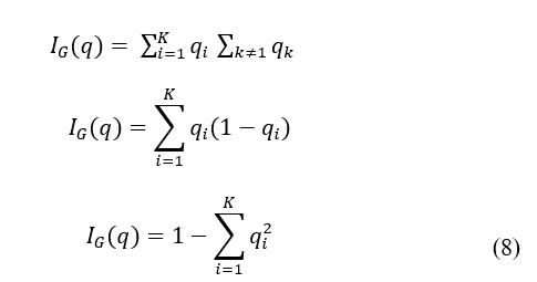
In the CART algorithm, the splitting process (or decision-making process at each step) is the most significant step of the training phase for machine learning. There are several criterions for the task. For example, Gini criterion (for CART) and Information entropy criterion (for C4.5) are widely used. Gini; a statistical measure which can be calculated by summing the random variable’s probability  (where  is the index for a random variable).

In order to calculate the Gini index for a set of features/attributes with  classes [47], let’s assume that and let  be the fraction of the items labelled with class  in the set. Accordingly, the set of equation is given by  (8).

3.4.  Dataset Preprocessing & Attack Types

Therefore, it can be seen that the Gini index  for a particular labelled item is a function of the sum of all probabilities in the tree. Research literature and various researchers discussion on blogs [48] [49] indicate that CART and C4.5 algorithms provide robust classification in application domains such as health care, marketing, financial forecasting and cyber security systems. The main advantage of the CART algorithm is that it does not have logarithm calculation in Gini index that makes the algorithm faster and efficient than the C4.5 algorithm.

The first dataset used in this research was obtained from the Cyber Range Lab of the Australian Centre for Cyber Security (ACCS) [19]. In this dataset, a hybrid of real modern normal activities and attack behaviors were generated. This dataset contains a total of forty-seven features and contains around 2.5 million sample data [19] [20]. It consists of such type of attacks like Fuzzers, Analysis, Backdoors, DDoS, Exploits, Generic, Reconnaissance, Shellcode, Worms & normal data samples with labels.

In the UNSW dataset, 47 columns represent attributes/features. Each recorded sample consists of attributes of different data forms like binary, float, integer and nominal. The attack data samples are labelled as ‘1,’ and normal data samples are labelled as ‘0’. Some of the feature data sample values are categorical values. For example, source IP address, destination IP address and source port number. Also, some other feature data sample values are continuous variable. For example, source bits per second, source jitter, and source TCP windows advertisement value. For preprocessing purpose, the features which values are categorical values were assigned a key value and stored in a dictionary. In the dictionary object, any values can be stored in an array, and each recorded item is associated with the form of key-value pairs. Furthermore, all the data samples were normalized using the following normal feature scaling process    (9):

The  is the normalized value and  is the original value. The file was saved into a text file for SVM input. In this way, all the data samples were preprocessed in the same pattern.

The total number of data sample in this dataset is 2,537,715 in which around 2.2 million is normal data samples the rest of the sample is attack data samples. In this dataset, the ratio of the normal and abnormal behavior is 87:13. Total normal data samples are 22,18,764, and total attack samples are 321,283.

The second dataset used in this research paper was collected from Canadian Institute of Cyber Security Excellence at the University of New Brunswick [21] upon request. The dataset is named as CIC IDS 2017, which is an Intrusion detection and evaluation dataset specially designed by collecting real-time traffic data flows over seven days that contains malicious and normal behaviors. In this dataset, there are over 2.3 million data samples, and among them, only 10% represents attack data samples. There are 80 network flow features in this data set.

The traffic data samples contain eight types of attacks namely Brute Force FTP, Brute Force SSH, DoS, Heartbleed, Web attack, Infiltration & DDoS [21]. This dataset is one of the richest datasets used for Network intrusion detection research purposes around the world [50]. The goal of using this data set is to evaluate how the proposed method works on different datasets.

4.      Proposed Algorithm

The steps of the proposed algorithm are listed below:

1. Define the number of features, N from the feature space.
2. Select the SVM parameter (Gamma, coef (), nu).
3. Define Number of Cooling (nCL) and Equilibrium loop (nEL).
4. Cooling loop Starts {i=1 to nCL}.
   1. Select n sub-features from the set
   2. Define an array D_R_array of size 10.
5. Equilibrium-loop starts { =1 to nEL}.
6. Train the SVM with the only selected feature.
7. Test the learning performance of SVM.
8. Store the solution in D_L
9. A small random perturbation of the features
10. Repeat steps 5a & 5b
11. Save the Solution in D_R
12. DR_array [ %10] = D_R
13. if 10 and Standard Deviation (D_R_array)
    1. Break from Equilibrium and Continue to Cooling loop
14. If D_R > D_L, then D_LßD_R
15. Else
    1. Find the Probability of Acceptance P
    2. Generate Random Number R
    3. If P > R, D_LßD_R
    4. If P < R, Check if number of Equilibrium loop (nEL)==0
    5. e) If (nEL)! =0, repeat 5(d), 5(e), 5(f)
    6. f) Else If (nEL)==0, Then D_LßD_R
16. Else If (nEL)==0, Reduce Temperature.
17. Equilibrium Loop Ends
18. Check Number of cooling loop (nCL)==0?
19. If (nCL)==0, Done

Else repeat procedure 4.

The proposed scheme defines the number of features in the dataset. Furthermore, the SVM parameters (Gamma, coef (), nu), Number of cooling loops (nCL), and number of equilibrium loops (nEL) are defined. At first, in the cooling loop,  number of features among  features are randomly selected (as initially, it does not know where to start with) where .  Then it moves inside the equilibrium loop, and trains the SVM with the selected  number of features and tests the learning performance of SVM. Then the algorithm saves the solution in DL. This solution is considered as an initial solution, and the goal of this loop is to find a best solution for the given temperature. A small random perturbation of the currently held features is made (seems like a random walk in the feature space) to create a new possible solution, because it is believed that good solution is generally close to each other but it is not guaranteed. The algorithm stores the solution in DR. If the cost of the new candidate solution is lower than the cost of the previous solution, then the new solution is kept and replaces the previous solution. Also, if the solution remains within  and factored by ten times in a row, the algorithm will terminate the current equilibrium loop and will check the cooling loop (if nCL  and continue another equilibrium loop to save time, as, it is assumed the algorithm is trapped in a local minimum solution. Sometimes the random perturbation results in worse solution; then, the algorithm decides to keep or discard the solution, which depends on an evaluation of the probability function. In case that the new solution is worse than the previous one then, the algorithm generates a random number R and compares with the probability function. If , the algorithm keeps the worse solution and if , then the algorithm checks whether it has reached the defined number of equilibrium loops or not. If (nEL)==0 then it moves out from the equilibrium loop to cooling loop and restarts the above described procedure again from the cooling loop. If (nEL)! = 0, then the algorithm starts from random perturbation inside the equilibrium loop and performs the procedure again. When the number of cooling loop reaches zero, then algorithm terminates and provide a meaningful solution [51]. This procedure is consuming less time and does not need and specific hardware configuration.

Table 1. 2-feature subset combinations.

#	Features in this Combination [19] [20]
1	·        The IP address of Source. ·        Service used (HTTP, FTP, SMTP, ssh, DNS, FTP-data, IRC and (-) if not much-used service)
2	·        Number of connections of the same source IP and the destination IP address in 100 connections according to the uncompressed content size of data transferred from the HTTP service last time. ·        Destination interpacket arrival time (mSec)
3	·        Source TCP based sequence Number. ·        Some flows that have methods such as Get and Post in HTTP service.
4	·        Destination TCP based sequence Number. ·        Mean value of the flow packet size transmitted by the Destination
5	·        Actual uncompressed content size of data transferred from the HTTP service ·        Number of connections is the same destination address & the source port in 100 connections according to the uncompressed content size of data transferred from the HTTP service.
6	·        Source Jitter (mSec). ·        Source retransmitted packet.
7	·        Mean of the flow packet size transmitted by the destination ·        Total packet count from Source to destination.
8	·         Destination bits per the second. ·         Source interpacket arrival time (mSec).
9	·        TCP connection setup time, the time between the SYN_ACK and the ACK packets. ·        Actual uncompressed content size of the data transferred from the server’s HTTP service.
10	·        Source interpacket arrival time (mSec) ·        Mean of the flow packet size transmitted by the destination.

This algorithm does not search the whole work/feature-space for reaching the global optimum solution. As a result, a small amount of time is required to provide a reasonable solution. It performed relatively well in large datasets. The efficacy of the proposed solution depends on the selection of essential features that help the intrusion detection process to detect an anomaly accurately.  To assure that the algorithm provides a better solution compared to other machine learning methods, it has been tested on two different types of datasets, which was explained in the previous chapter.

5.      Experiments and Results

This section is divided into several sections. Both datasets contain different numbers of features. The results are discussed in details using multiple feature subsets (Ex. 2, 3, 4 and 5).

5.1.  Simulation Setup and outcomes of the Proposed Algorithm (2 features UNSW Dataset)

In this simulation setup, the proposed algorithm has been applied taking two feature subsets as an initial approach. Afterwards, we will try three, four and five feature subset combinations to inspect how the algorithm performs if the number of features increases in a subset. Table 1 shows 2-feature subset combinations:

The detection accuracy of the proposed method versus the feature combination is shown in Fig. 1.

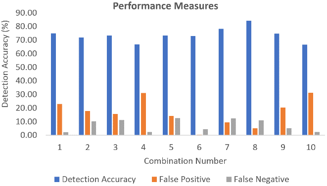
Figure 1. Detection Accuracy, False Positive and False Negative for 2 feature subset combination.

Table 1 shows the combination number denotes which two features were selected for that combination. The proposed algorithm achieved a detection accuracy recorded as 84.14% when combination number 8 was selected. The lowest detection accuracy among the given results was recorded as 63.56% for combination number 10.

Considering only two feature subsets provided a high false positive and false negative rate of 5.09% and 10.77% respectively. Upon checking the ROC curve (Fig. 2), these combinations provided poor AUC value. It may be caused by taking an imbalanced number of features. The feature subset is selected by the SA process, which may not be linearly separable on the classification space. Using a non-linear typical decision boundary will require more computational efforts than fitting linear decision boundary. Thus, increasing the dimension (or features) may provide better results compared to the 2-feature subsets, as it may allow the hyperplane to separate the data.

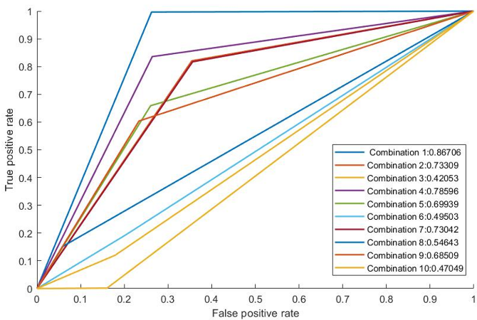
Figure 2. RoC analysis 2-feature subset.

The F1-score is a statistical analysis of binary classification and a measure of precision. The F1-score can be described as a harmonic mean of the precision and recall, where an F1-score reaches its best value at one and worse at 0. Precision is the ratio of correctly projected positive annotations to the total projected positive annotations, whereas recall is the ratio of correctly predicted positive annotations to all annotations in the actual class. The reason why harmonic mean is considered as the average of ratios or percentages is considered. In this case, harmonic mean is more appropriate then the arithmetic mean. As shown in fig 2Error! Reference source not found., we plotted the F1-score for each combination of 2-feature sets (Table 1). As shown, the F1-score is quite low, except for combination 8, where it achieved almost 0.92; otherwise it was an average of about 0.81. Based on our other subsequent experiments, these values were deemed too low, and more features per combination were apparently required to achieve better F1-score results.

5.2.  Simulation Setup and outcomes of Proposed Algorithm (3 features UNSW Dataset)

In the previous section, the proposed algorithm was tested and results analyzed for two feature subsets. While this seemed fine for an initial approach, we found the F1-score results to be quite low, and so we now present results for more features per combination. In particular, Fig. 3 shows the 3-feature subset combinations. Afterwards, we present the results for three, four and five feature subset combinations to inspect how the algorithm performs.

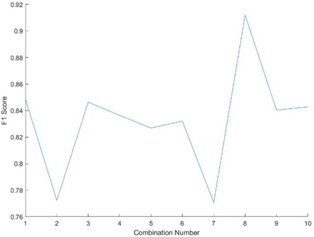Figure 3. F1-score of the 2-feature subset combination.

Table 2. 3-feature Subset Combination.

#	Features in this Combination [19] [20]
1	·        The IP address of Source ·        Service used (HTTP, FTP, SMTP, ssh, DNS, FTP-data, IRC and (-) if not much-used service). ·        Source packets retransmitted or dropped.
2	·        Source TCP window advertisement value ·        No of connections of the same source IP and the destination IP address in 100 connections according to the uncompressed content size of data transferred from the HTTP service last time ·        Destination interpacket arrival time (mSec)
3	·        Source TCP based sequence Number ·        Some flows that have methods such as Get and Post in HTTP service. ·        No. of connections of the same destination address in 100 connections according to the uncompressed content size of data transferred from the HTTP service last time
4	·        Destination TCP based sequence Number. ·        Source TCP based sequence Number. ·        Mean value of the flow packet size transmitted by the Destination.
5	·        Actual uncompressed content size of data transferred from the HTTP service. ·        TCP base sequence number of destinations. Number of connections is the same destination address & the source port in 100 connections according to the uncompressed content size of data transferred from the HTTP service
6	·        Source Jitter (mSec). ·        Source retransmitted packet. ·        Destination bits per second.
7	·        Source Jitter (mSec) ·        Mean of the flow packet size transmitted by the destination ·        Total packet count from Source to destination
8	·        Destination bits per the second ·        Source interpacket arrival time (mSec) ·        Number for each state dependent protocol according to a specific range of values for   source/destination time to live
9	·        TCP connection setup time, the time between the SYN_ACK and the ACK packets. ·        Source bits per second ·        Actual uncompressed content size of the data transferred from the server’s HTTP service.
10	·        Destination Interval arrival Time ·        Source interpacket arrival time (mSec) ·        Mean of the flow packet size transmitted by the destination.

A list of ten combinations has been shown, and each combination contains three features. The mechanism of the initial approach in the research was that it takes three features at a time and provide an output. Afterwards, it discards the results and tries another randomly selected feature combination. Trying all possible combination implies that it leads to an exhaustive search and takes a huge amount of computational resources and consumes more time. Further, it will more time if a large number of features are considered. However, in the proposed algorithm, the annealing process starts selecting a random set of three features as the first step as it has to begin somewhere randomly. Then the SVM is trained only with these three features, and the generated output is saved. It is considered as a first initial solution. A small random perturbation is made to the current solution changing one or two features because it is assumed that good solutions are generally close to each other, but it is not guaranteed as the best solution. Sometimes the newly generated solution results in a better solution than the algorithm keeps the new solution. If the newly generated solution is worse than the current solution, then the algorithm decides whether to keep or discard the worse solution, which depends on the evaluation of the probability function      (7). The higher temperature in the annealing process, it is more likely the algorithm will keep the worse solution. Keeping the worse solution allows the algorithm to explore the solution space and to keep it within the local optima. Also neglecting a worse solution lets the algorithm to exploit a local optimum solution, which could be the global solution for that temperature.

The detection accuracy of the proposed method versus to the feature combination is shown in Fig. 4. In Fig. 3, the combination number denotes which three features were extracted for that combination.

The proposed algorithm achieved a detection accuracy recorded as 98.32% when combination number 8 was selected (Fig. 3). This combination contains three essential features, such as destination bits per second, source interpacket arrival time (mSec), and number of each state dependent protocol according to a specific range of values for source/destination time to live value. The lowest detection accuracy among the given results was recorded as 72.08% when combination number 4 was used. Comparing with the 2-feature subset combination results, we can infer that as another dimension was introduced, the linear classification technique worked better.

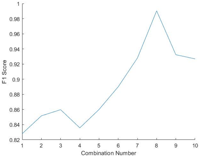
Figure 4. Detection Accuracy, False Positive and False Negative for 3-feature subset combination.

Furthermore, the performance metrics of the proposed algorithm was investigated. The false positive refers to a situation that the system incorrectly identifies an object as a positive (attack), which, however, is not an attack and is a normal (non-attack) object. The false negative refers to a situation that the system incorrectly identifies an object as a negative (non-attack), which however is an attack. Also, the percentage of false positives and the percentage of false negatives are shown for the proposed scheme. The false positives and false negatives were recorded as 1.49% and 0.19% respectively, for combination number 8. Therefore, it can be inferred that, if the correlative features are extracted, the false positive and negative rate decreases, it may provide a relatively better solution for intrusion detection.

In Fig. 5 the receiver operating characteristic curves for the proposed schemes are presented.

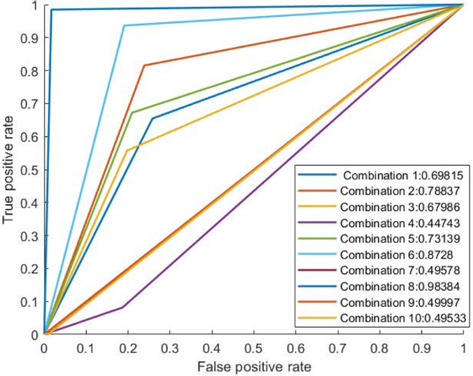
Figure 5. RoC curve analysis for 3-feature subset.

In a real-world scenario, the misclassifications costs are difficult to determine. In this regard, the ROC curve and its related measures, such as AUC (Area under Curve) can be more meaningful and deemed as vital performance measures. As shown in the figure, it is seen that the performance output is much better than the previous performance with 2-feature combinations. The combination number 8, which contains features such as Destination bits per second, Source interpacket arrival time (mSec), Number of each state dependent protocol according to a specific range of values for source/destination time to live value, provided much better reasonable output. The AUC of that combination is 0.98384, which is closer to one, which presents a better solution in contrast with the other possible solutions.

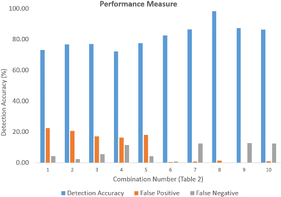
Figure 6. F1-score 3-feature subset.

The F1-score of the different combinations is shown in Fig. 6. Note that the combination number 8 achieved the highest F1-score of 0.99.

Fig. 7 demonstrates the detection accuracy of the proposed scheme increases or decreases along as the number of iterations varies.

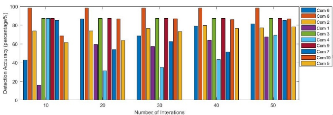
Figure 7. Detection accuracy difference versus number of iterations.

A cross-validation mechanism was used to assess the predictive performance of the model to evaluate how good the model works on a new independent dataset (using resampling randomly). It is seen that combination 1 (violet) started with very low detection accuracy, but while iterating multiple times the detection accuracy increased, and an average of those accuracies provide a well reasonable solution for that combination.

However, combination 8 (light brown) started with higher accuracy, and while multiple iterations are running, it kept almost the same as it is and an average of those accuracies has been considered. Furthermore, the combination number 4 (sky blue) stared with higher accuracy but while multiple times iterations the accuracy went down and suddenly went up. An average of those accuracies has been considered. Taking averages of the detection accuracies allows the algorithm to be more confident on the provided output. The proposed scheme does not take too long to converge to the local optima (which can be the global optima) but provides a reasonable detection accuracy over short possible time, depending on the system resources.

To evaluate whether the algorithm works as intended, unit testing was performed, and the detection accuracy was measured for different numbers of thermal equilibrium loops, as shown in Fig. 8.

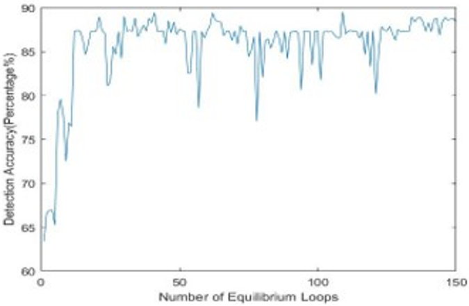
Figure 8. Performance of the proposed scheme for varying numbers of thermal equilibrium loops.

The annealing process starts at a random direction as it does not know which direction to start with and the first solution is considered as the initial solution. On each iteration, a random perturbation in the solution space is performed, and a new solution is generated. Comparing with the previous solution it is better or worse, it keeps the better solution and marches forward, as it is believed the good solutions may be nearby. Fig. 8 shows that the algorithm starts with a low detection accuracy and marching forward it is going towards higher accuracy. While going forward, it seems that it may have found worse candidate solution (the down hikes on the Fig. 8 but keeping the worse solution allows the algorithm to explore more in the solution space to reach an optimum solution. These observations of the results verify that the algorithm is performing the way it supposed to perform.

As the algorithm starts from a random direction, provides an initial solution, takes random perturbation, and generates another new solution, a scenario is visualized that sometimes the detection accuracy of the old candidate solution and new candidate solution is quite close enough like a slight difference of some percentage. For the time being, it is being trapped on that local optima. So, to save more time and speed up, the algorithm is designed in such way that, if the difference of the accuracy of the old candidate solution and new candidate solution is around ±2% and ten times in a row, the algorithm will terminate that equilibrium loop. Subsequently, the algorithm will go to the next cooling loop (if nCL!=0) and start another inner loop and continue. Fig. 9 shows that inside the equilibrium loop iteration number approximately from 139-150, the detection accuracy stays between 86%-87% for the time being, and it detected an accuracy difference of ±2% ten times in a row. Therefore, the proposed method will terminate the current equilibrium loop, decrease temperature and start the next cooling loop if nCL!=0.

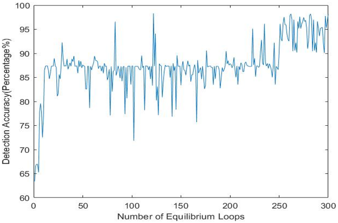
Figure 9. Detection accuracy of the equilibrium loops.

In a nutshell, the proposed algorithm starts from a random path to find an initial solution (initial 3-feature combination) and takes small random walk in the feature space (changing 1 or more features) and compares with the previous solution that allows the algorithm to converge faster to the local optima which may likely be a local optimum solution.

5.3.  Simulation Setup and outcomes of Proposed Algorithm (4 features UNSW Dataset)

Next, the performance of the algorithm was evaluated taking four and five features in a subset. The algorithm will initiate with a four-feature subset combination. Furthermore, the outcomes with be compared with the 3-feature subset combinations. The comparison allows us to determine how the algorithm performs when the number of features increases. The number of training samples and the number of testing samples were kept the same as previous. Table 3 shows the combination of four features.

Table 3. 4-feature subset combination.

#	Features Taken [19] [20]
1	·        Source IP address ·        Source packets retransmitted or dropped ·        Destination to the source packet count ·        No of connections of the same source address (1) and the destination port (4) in 100 connections according to the last time (26).
2	·        Source inter-packet arrival time (mSec) ·        Destination inter-packet arrival time (mSec) ·        If the FTP session is accessed by user and password then 1 else 0. ·        No. of connections that contain the same service (14) and source address (1) in 100 connections according to the last time (26)
3	·        Source to destination time to live value ·        Source TCP sequence number ·        No. of flows that has methods such as Get and Post in HTTP service. ·        No of flows that have a command in an FTP session.
4	·        Destination IP address ·        Destination TCP window advertisement value ·        Source TCP sequence number ·        d. Mean of the flow packet size transmitted by the destination
5	·        The content size of the data transferred from the server’s HTTP service. ·        No of connections of the same destination address (3) and the source port (2) in 100 connections according to the last time (26). ·        No. of connections that contain the same service (14) and destination address (3) in 100 connections according to the last time (26). ·        d. Source TCP window advertisement value
6	·        Source jitter (mSec) ·        Destination bits per second ·        No. of connections that contain the same service (14) and source address (1) in 100 connections according to the last time (26). ·        d. No of flows that have a command in an FTP session.
7	·        Source to destination packet count ·        Mean of the flow packet size transmitted by the destination ·        The time between the SYN_ACK and the ACK packets of the TCP. ·        d. No. of flows that has methods such as Get and Post in HTTP service.
8	·        No. for each state according to a specific range of values for source/destination time to live value ·        Destination bits per second ·        Source bits per second ·        d. The time between the SYN and the SYN_ACK packets of the TCP.
9	·        The content size of the data transferred from the server’s HTTP service. ·        Source bits per second ·        HTTP, FTP, ssh, DNS., else (-) ·        Mean of the flow packet size transmitted by the destination.
10	·        No. for each state according to a specific range of values for source/destination time to live value ·        Source bits per second ·        Destination jitter (mSec) ·        d. If the source equals to the destination IP addresses and port numbers are equal, this variable takes value one else zero

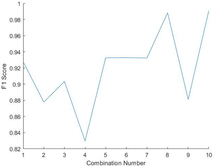Figure 10. Detection accuracy for the four-feature combination.

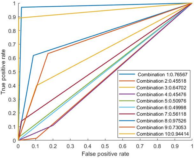Figure 11. RoC curve and AUC for the four-feature combination.

Evaluating the above results, we can see that taking four features increases some of the combinations’ detection accuracies. For example, comparing 3-feature combination number 8 of Fig. 3 with 4-feature combination number 8 of Table 3, the detection accuracies were 98.32% and 97.97% respectively, resulting in a 0.35% positive difference in detection accuracy. The algorithm kept Destination bits per second and Number of each state dependent protocol according to specific range of values for source/destination time to live value features steady and while taking 4 feature combination it selected two features such as Source bits per second, the time between the SYN and the SYN_ACK packets of the TCP which allowed the algorithm to provide a reasonable solution. Therefore, the 3-feature subset combination 8 is better regarding accuracy, time consumption, low false positive, higher AUC value and higher F1-score compared to 4-feature subset combinations 8.

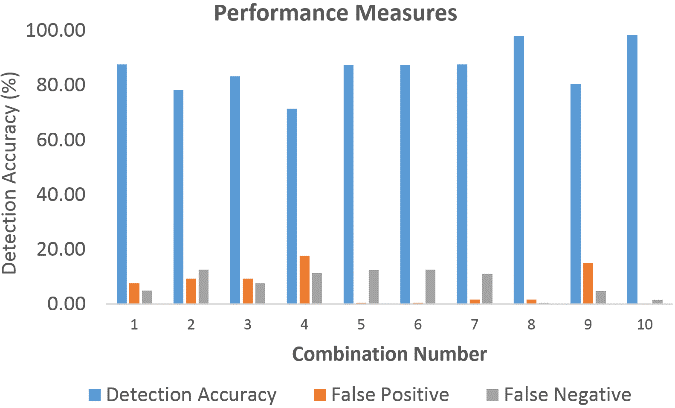Figure 12. F1-score for the 4-feature subset combination.

However, if we look at the combination number 10 when 4 features are selected such as No. for each state according to specific range of values for source/destination time to live value, Source bits per second, Destination jitter (mSec) and If source equals destination IP addresses and port numbers are equal-this variable takes value 1 else 0, provided a detection accuracy of 98.39% which is the highest accuracy the algorithm provided. Comparing with the 3-feature combination number 8, the difference of detection accuracy is 0.07% only (3 feature detection accuracy is 98.32%). Increasing dimension (SA) allowed the feature space hyperplane to separate the normal and attack sample more precisely for this particular feature subset compared to 3-feature combination number 8 (Fig. 3). However, regarding AUC, ROC, false negatives and F1-score the 3-feature combination number 8 (Fig. 3) overall was the most reasonable solution here.

For further evaluation of the performance to determine the effect of providing more features, we have analyzed the behavior of the proposed scheme taking five feature subset combinations. It is described in the following section.

5.4.  Simulation Setup and outcomes of Proposed Algorithm (5 features UNSW Dataset)

In this setup, five feature subset combination were considered, and the performance of the proposed method was evaluated regarding detection accuracy, false positive and negative, F1-score, ROC characteristics, Area under the curve.

Analyzing the performance of the proposed scheme while considering a 5-feature subset, the detection accuracy of most of the feature combinations reduced significantly. This reduction in detection may be caused because of insignificant and irrelevant dimensions or features in the dataset were considered in a feature subset. The algorithm may not have been trained appropriately due to a large number of dimensions considered in this step. As a result, the algorithm was unable to provide a reasonable solution in most of the feature combinations.

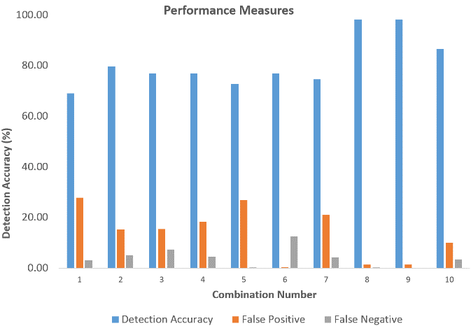Figure 13. Detection Accuracy for 5 feature subset combination.

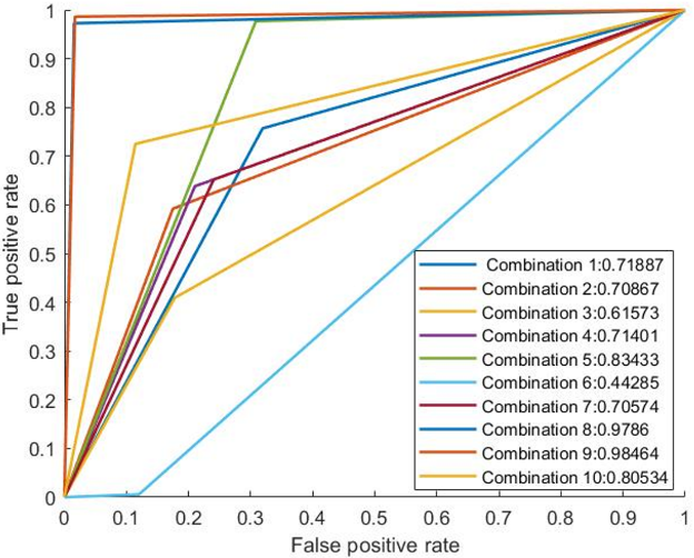Figure 14. RoC Analysis of 5-feature subset (UNB Dataset).

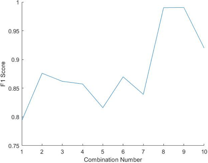Figure 15. F1-score for 5 feature subset combination.

However, it is observed that combination number 8 and 9 provided a better detection accuracy compared to other feature subset combinations. The 5-feature subset (combination 9) provided an accuracy of 98.34%, which is only .02% higher than the 3-feature subset (combination 8, Fig. 3). The false positive and false negative rate of combination 3-feature subset (combination 8, Fig. 3) is 1.49% and 0.19%, and 5-feature subset (combination 9) is almost same as 1.49% and 0.17% respectively. There were no significant changes in the parameters. The difference of the AUC value of 5-feature and 3-feature subset is 0.001, which is very negligible. Regarding F1-score, the 3-feature subset combination 8 (Fig. 3) provided better outcomes compared to 5-feature subset combinations. It is obvious that if the 3-feature subset is considered, the algorithm will take a shorter time to provide a solution compared to with that of 5-feature subset combination.

5.5.  Simulation Setup and outcomes of Proposed Algorithm (3 features UNB Dataset)

The dataset collected from Canadian Information Security Center of Excellence at the University of New Brunswick (upon request) to analyze the behavior of the proposed scheme. Recently in 2017, they experimentally generated one of the richest Network Intrusion Detection dataset containing 80 network flow features, which were generated from capturing daily network traffic. Full details were provided on [21]. This paper also provided information that what features are very much significant to detect a specific type of attack. This dataset was considered to evaluate that how the proposed scheme will work on an entirely different dataset and how much confidence the algorithm has on its provided outcomes.

This dataset also contained some features similar to the previous UNSW dataset. The dataset contains categorized and continuous variables. It was preprocessed similar way with the feature scaling process equation 12. Detailed experimental results are discussed below.

Table 4. 3-feature subset combination for UNB dataset.

#	Features in this combination [21]
1	·      backward packet length min ·      total length flow packets ·      c. flow inter-arrival time min
2	·      flow inter-arrival time min ·      Initial win forward bytes ·      Flow inter-arrival time std.
3	·      flow duration ·      Active min of bytes ·      the active mean of flow bytes
4	·      backward packet length std ·      Length of forwarding packets ·     sub-flow of bytes
5	·      avg packet size ·      Backward packet length std ·     mean of active packets
6	·      flow inter-arrival time min ·      Backward inter-arrival time means ·      initial win forward bytes
7	·      forward push flags ·      Syn flag count ·      c. back packets/s
8	·      backward packet length std ·      Avg packet size ·      flow inter-arrival time std
9	·      forward packet length mean ·      Total length forward packets ·      sub-flow forward bytes
10	·        initial win forward bytes ·        Backward packets/s ·        flow inter-arrival time std

Upon evaluation of the above outcomes, it is observed that the detection accuracy of the algorithm increased in some feature combinations and was able to provide a detection accuracy of 96.58% (Combination 8). The Receiver operation characteristics show that the algorithm was provided with a reasonable AUC value (combination 8) compared to other methods discussed previously. In the research paper [21] Table 3, the author provided a particular set of feature set which is more significant detecting a particular intrusion such as for the detection of a DDoS attack, backward packet length, average packet size and some inter-arrival time of the packets, flow IAT std. Now the proposed scheme selected three features out of the four features (mentioned in that paper by the author) shown on combination number 8 as the evaluation was done taking three features at a time. These three features provided an accuracy of 96.58%, an AUC value of 0.92199 and an F1-score of 0.980416. If the full dataset with all 80 features [21] were available, then the results might get better than the current one.

Figure 16. Detection accuracy for the 3-feature subset combinations (UNB Dataset).

Figure 17. RoC Analysis of 3-feature subset (UNB Dataset).

F1-score for the 3-feature subset (UNB Dataset).

Upon evaluation of the above outcomes, it is observed that the detection accuracy of the algorithm increased in some feature combinations and was able to provide a detection accuracy of 96.58% (Combination 8). The Receiver operation characteristics show that the algorithm was provided with a reasonable AUC value (combination 8) compared to other methods discussed previously. In the research paper [21] Table 3, the author provided a particular set of feature set which is more significant detecting a particular intrusion such as for the detection of a DDoS attack, backward packet length, average packet size and some inter-arrival time of the packets, flow IAT std. Now the proposed scheme selected three features out of the four features (mentioned in that paper by the author) shown on combination number 8 as the evaluation was done taking three features at a time. These three features provided an accuracy of 96.58%, an AUC value of 0.92199 and an F1-score of 0.980416. If the full dataset with all 80 features [21] were available, then the results might get better than the current one.

5.6.  Performance Comparison

In this section, we have analyzed the performances of the proposed method in detail in comparison with general SVM and Decision tree-based detection method concerning the performance matrices.

In the initial approach of this research [52] was at first the algorithm selects  features using random combination from the  features from the dataset. Then it selects the SVM parameters and trains the classifier. Afterwards, the algorithm rum SVM on the test data samples and tries to identify the positive and negative training examples. It discards the previously selected feature set, takes another random combination of features, and continue the process until all possible combinations (depending on the number of feature input) are completed. This process leads the algorithm to perform an exhaustive search in the whole workspace trying all possible combinations leading to a combinatorial optimization problem. In combinatorial optimization, it is very difficult to determine how many number or which feature combination set will provide a reasonable solution minimizing the cost and decision-making time. When the number of features in a subset increases, the number of combinations also increases exponentially. The performance of the initial algorithm is presented below where the algorithm provides outputs of different random feature combinations and its very random.

We can see from Fig. 18 that the output of different 3-feature subset is very random and the algorithm is performing an exhaustive in the whole workspace to provide an optimal solution.  For more substantial dataset form the current one, it will be much exhaustive for the algorithm to provide a solution. Thus, the combinatorial optimization exists in this scenario.

Figure 18. Performance of the initial approach (exhaustive search).

In contrast with the above discussion, the proposed algorithm does not search the whole workspace for finding a solution rather than it starts from a random direction at the beginning as initially, the algorithm does not know which way to start from. In the outer loop known as known as a cooling loop of SA, depending on the feature input (2,3,4 or more) the algorithm selects a random subset of feature to start with and trains the SVM (cost function of SA) only with the selected features at that temperature. Inside the equilibrium loop, the first solution is considered as the initial one. The cost function determines the goodness of the solution. Afterwards, the algorithm takes a small random perturbation to create a new candidate solution because it is assumed that good solutions are generally close to each other, but it is not guaranteed as the best optimal solution. If the newly generated solution is worse than the current solution, then the algorithm decides whether to keep or discard the worse solution, which depends on the evaluation of the probability function (equation 7). After running the inner loop many times, wherein each loop it takes a new better solution or keeps a worse solution, the algorithm may be viewed as taking a random walk in the solution space to find a sub-optimal solution for the given temperature. The performance inside the equilibrium loop is shown in fig. 18.

If the comparison is made between Fig. 18 and 19, we can see that the proposed method outcome does not show high variance like the Fig. 18 (variance of the Fig. 18 is ± 3.9% and the current is ±1.9%). The initial algorithm is performing an exhaustive search over the whole workspace, finding the global solution whereas the proposed method does not search the whole workspace, and providing the best possible local optimum solution for the given temperature, which may be the global optimum solution. The proposed method consumes less time and less computational cost compared to the exhaustive search method.

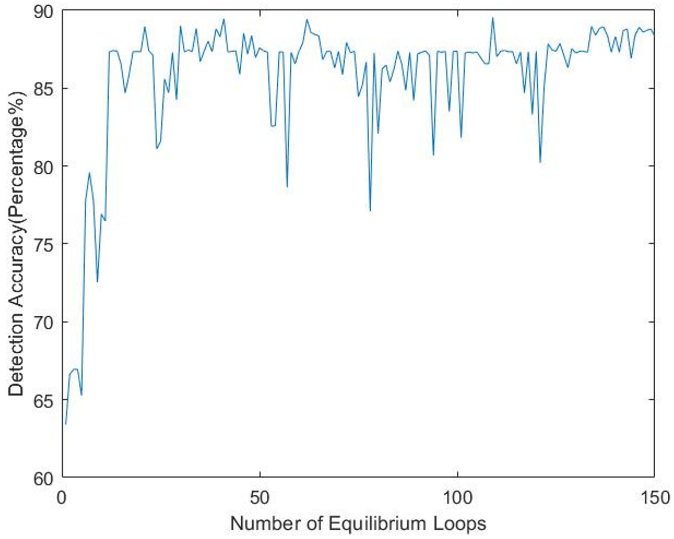Figure 19. Performance of the Proposed method.

Sometimes inside the equilibrium loop, it is observed that the difference of the solution outcomes is not that significant. After visual observation of the cost function inside the equilibrium loop, it is observed that the output of the variance of the outcomes lies below 3%. It looks like the algorithm is trapped inside that local optimum solution until the inner loop ends. To save time and speed up the performance, the algorithm is designed in such way that, if the difference of the accuracy of the old candidate solution and new candidate solution is around ±2% factored by ten times in a row, the algorithm will terminate that equilibrium loop. Subsequently, the algorithm will go to the next cooling loop (if nCL! = 0) and start another inner loop and continue. A general standard deviation method was applied to the steps of the algorithm in fig. 20.

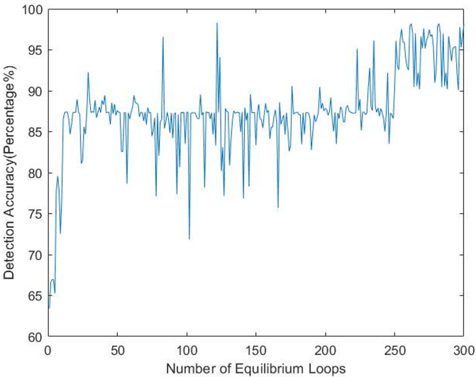Figure 20. Termination of equilibrium loop.

If another dataset is considered which contains many features, the number of combinations will increase, and the initial algorithm will take more time, and the computational cost will be more. The proposed method does not try all possible combinations to provide a solution. It provides the best local optimum solution for the given temperature, and it may be the global optimum solution. The proposed methodology can be considered as a general methodology and can be applied t o other sectors to solve the feature extraction combinatorial optimization problem to save time and computational resources. Notably, the proposed method saves time and computational resources and provides a better outcome compared to the general SVM based exhaustive search method.

5.7.  Performance comparison with Decision tree-based method

In this section, we have evaluated the performance of a decision tree-based method and compared the outcomes with the proposed method. There are several algorithms based on decision trees like C4.5, CART, and ID3. In this research, we have applied the CART (Classification and Regression Tree) algorithm [44] for classification purposes. For a fair comparison with the proposed method, the same feature set was applied to the decision tree-based method on the same dataset (UNSW dataset). Furthermore, the decision tree-based methodology was applied in the second dataset (UNB dataset) to evaluate how the decision tree algorithm performs on two different types of dataset. We have evaluated the performance of a decision tree-based method on same 3-feature subset combinations (Fig. 3 for UNSW dataset and Table 4 for UNB dataset).

In the Fig. 20, the detection accuracy, false positive and false negative rate were observed when the CART algorithm was applied on the UNSW dataset. The 3-feature subset combinations were kept same as previous. Let us compare the outcomes of the decision tree method with the 3-feature subset combination outcomes of the proposed method.

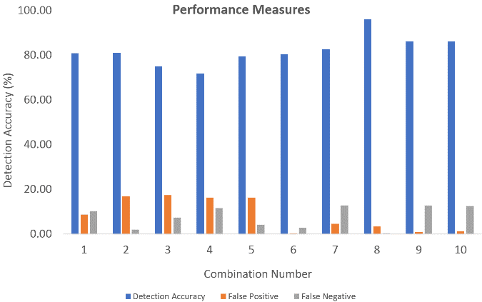Figure 21. Performance metrics of the decision tree-based method (UNSW dataset).

Upon evaluation of the performance metrics of the decision tree-based method and the proposed SA-SVM based method we can see that, combination number 8 with three feature subsets such as Destination bits per the second, Source interpacket arrival time (mSec) and No. for each state dependent protocol according to a specific range of values for source/destination time to live value, the detection accuracy of the decision tree is 96.16%, false positive and false negative rate is 3.45% and 0.39%, whereas the proposed method provides a higher detection accuracy of 98.32%, false positive rate of 1.49%, false negative rate of 0.19%. The proposed method provided better results compared to the decision tree-based method in most of the subset combinations. These empirically validated outcomes show that the proposed method outperforms the decision tree-based method.

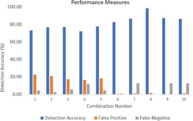Figure 22 Performance metrics of the proposed method (UNSW dataset).

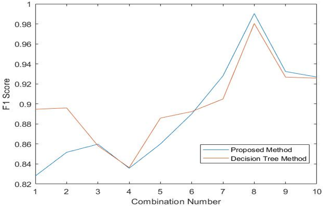Fig. 23 represents the F1-score comparison between the decision tree-based method and the proposed method.

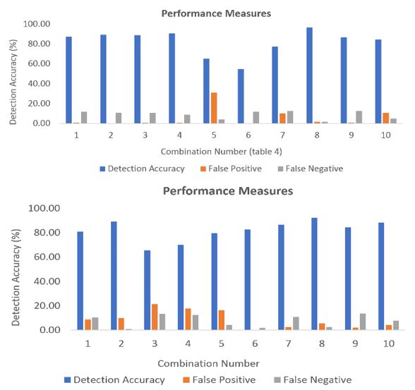Figure 24. F1-score comparisons (UNSW dataset).

The F1-score is a statistical measure of tests accuracy that measures how accurate is the classifier; meaning how many instances it classifies correctly. It also tells how robust the classifier is meaning it does not miss a significant number of instances. We can see from Fig. 24 that combination 8 (Fig. 3) the decision tree-based method provided an F1-score of 0.980401 whereas the proposed method provided an F1-score of 0.990522. The proposed method provided higher F1-score compared to the decision tree-based method.

For further performance evaluation, the decision tree-based method was applied on the UNB 2017 dataset also, and the outcomes were compared with the proposed method. The three-feature subset was kept the same for the evaluation. We will analyze how decision tree performs on a different dataset.

In Fig. 24 the detection accuracy, false positive and false negative rate were observed when the CART algorithm was applied on the UNB dataset. The 3-feature subset combinations were kept same as previous. Let us compare the outcomes of the decision tree method with the 3-feature subset combination outcomes of the proposed method.

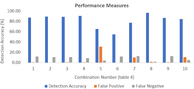Figure 25. Performance metrics of the decision tree-based method (UNB dataset).

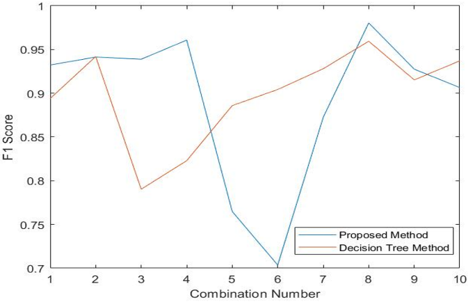Figure 26. Performance metrics of the proposed method (UNB dataset).

Upon analysis of the performance metrics of the decision tree-based method and the proposed SA-SVM based method on the UNB dataset, combination number 8 with three feature subsets such as flow inter-arrival time, flow back packet length, flow duration represents DDoS attack [76] the detection accuracy of the decision tree is 92.22%, false positive and false negative rate is 5.42% and 2.36%, whereas the proposed method provides a higher detection accuracy of 96.58%, false positive rate of 1.70%, false negative rate of 1.73%. The proposed method provided better results in contrast to the decision tree-based method in most of the subset combinations when a different dataset was used. These empirically validated outcomes show that the proposed method outperforms the decision tree-based method on UNB dataset also.

6.      Conclusions and Future Works

This paper provides a computationally intelligent approach, merging machine learning & combinatorial optimization, to provide a comparatively reasonable solution for optimum feature extraction from a large set of features, which is a difficult combinatorial optimization problem. The experimental results show that this proposed scheme provides better outcomes in comparison with other machine learning methods like Decision Trees and general SVM alone based approaches. As the results showed, this methodology performed effectively and efficiently in contrast with other machine learning methods while applying on different network intrusion datasets. Empirically validated outcomes show that the proposed method outperformed the Decision Tree and general SVM based solution concerning the performance metrics. The proposed algorithm provided an average detection accuracy of 98.32% with false positives and false negative rates of 1.49% and 0.19% respectively when a particular 3-feature subset was considered (Fig. 3). The receiver operating characteristics (ROC) shows a better view of the outcome regarding the AUC value of 0.98384, which is closer to one, an F1-score of 0.9905. This proposed scheme provides a reasonable solution for the feature extraction combinatorial optimization problem and does not require any specific hardware configuration.

Future works can be extended to enhance the performance of the algorithm and evaluate the effectiveness of the proposed scheme. The following are a few proposed extensions of future work:

1. In the proposed scheme Simulated Annealing is used for finding the best feature combination without trying all possible feature combination and SVM is used as the cost function. In this case, instead of Simulated Annealing, Genetic algorithms can be introduced to evaluate the performance of the proposed scheme. Also, Artificial Neural Networks can also be considered to differentiate the performances so we can be more confident about the outcomes that which algorithm performs better.

1. In this research, one of the feature columns was discarded named attack category, which specifies which type of intrusion it is. In the UNSW and UNB dataset, all the intrusions are labelled as one (regardless of their category), and regular traffic is labelled as logical 0. The proposed scheme can detect the intrusion with improved precision compared to other detection methods discussed but is unable to determine what type of intrusion it is. So, future works can include considering the attack categories so the algorithm will learn more and provide a particular set of significant features to detect a particular type of network attack.

1. To pre-process the data samples, the linear feature scaling process were considered. However, future work can introduce standardization method to preprocess the data samples and analyze the performances to differentiate how good/bad the algorithm performs if different scaling process is used.

Acquiring latest, real-time and effective network intrusion datasets is difficult. The proposed method is only tested on Network intrusion detection datasets from University of New South Wales, Australia and University of New Brunswick, Canada as these two institutions have generated the most recent intrusion detection upgraded datasets, which are being considered as one of the richest datasets. This new detection scheme may be used in other sectors like finance & economy, portfolio management, health analysis and fraud detection.  Therefore, as future work, this proposed method can be applied in different sectors and evaluate the performances to establish that this method is a generalized method and may be used towards any dataset to provide a reasonable solution for combinatorial optimization problem compared to other machine learning methods.

Conflict of Interest

The authors declare no conflict of interest.

1. “Challenges of Big Data analysis,” National Science Review, vol. 1, no. 2, p. 293–314, June 2014.
2. Alexandra L’Heureux, Katarina Grolinger, Hany F. Elyamany and Miriam A. M. Capretz, “Machine Learning with Big Data: Challenges and Approaches,” ” IEEE Access Journal, vol. 5, pp. 7776 – 7797, April 2017.
3. M. G. Kibria, K. Nguyen, G. P. Villardi, O. Zhao, K. Ishizu and F. Kojim, “Big Data Analytics, Machine Learning, and Artificial Intelligence in Next-Generation Wireless Networks,” IEEE Access Journal, May 2018.
4. J. J. Hopfield, “Neurons with graded response have collective computational properties like those of two-state neurons,” Proc. Natl. Acad. Sci. USA, vol. 81, 1984.
5. F. S. Girish Chandrashekar, “A survey on feature selection methods,” Computers & Electrical Engineering, vol. 40, no. 1, pp. 16-28, January 2014.
6. P. M. M. A. Pardalos, Open Problems in Optimization and Data Analysis, 2018.
7. Miloš Madi, Marko Kovačević and Miroslav Radovanović, “Application of Exhaustive Iterative Search Algorithm for Solving Machining Optimization Problems,” Nonconventional Technologies Review Romania, September 2014.
8. Cui Zhang , Qiang Li and Ronglong Wang , “An intelligent algorithm based on neural network for combinatorial optimization problems,” in 2014 7th International Conference on Biomedical Engineering and Informatics, Oct. 2014.
9. M. Chakraborty and U. Chakraborty, “Applying genetic algorithm and simulated annealing to a combinatorial optimization problem,” in Proceedings of ICICS, 1997 International Conference on Information, Communications and Signal Processing. Theme: Trends in Information Systems Engineering and Wireless Multimedia Communications, 1997.
10. X. Liu, B. Zhang and F. Du, “Integrating Relative Coordinates with Simulated Annealing to Solve a Traveling Salesman Problem,” in 2014 Seventh International Joint Conference on Computational Sciences and Optimization, July 2014.
11. M. Gao and J. Tian, “Network Intrusion Detection Method Based on Improved Simulated Annealing Neural Network,” in 2009 International Conference on Measuring Technology and Mechatronics Automation, April 2009.
12. R. D. Brandt, Y. Wang, , A. J. Laub and S. K. Mitra, “Alternative networks for solving the traveling salesman problem and the list-matching problem,” in Proceedings of IEEE International Conference on Neural Networks, 1998.
13. SUN Jian, YANG Xiao-guang, and LIU Hao-de, “Study on Microscopic Traffic Simulation Model Systematic Parameter Calibration,” Journal of System Simulation, 2007.
14. R. M. V. H. R. Z. W. P. M. Azencott, “Automatic clustering in large sets of time series,” in Partial Differential Equations and Applications, Springer, Cham, 2019, pp. 65-75.
15. Ping-Feng Pai and Wei-Chiang Hong, “Support vector machines with simulated annealing algorithms in electricity load forecasting,” Energy Conversion & Management, vol. 46, no. 17, Oct 2005.
16. J. S. Sartakhti, Homayun Afrabandpey and Mohammad Saraee, “Simulated annealing least squares twin support vector machine (SA-LSTSVM) for pattern classification,” Soft Computing, Springer Verlag, 2017.
17. P. J. Herrera, Gonzalo Pajares, María Guijarro and José Jaime Ruz, “Combining Support Vector Machines and simulated annealing for stereovision matching with fish eye lenses in forest environments,” Expert Systems with Applications, Elsevier, July 2011.
18. K. Murugan and Dr. P.Suresh,, “Optimized Simulated Annealing Svm Classifier For Anomaly Intrusion Detection In Wireless Adhoc Network,”
19. AUSTRALIAN JOURNAL OF BASIC AND APPLIED SCIENCES, vol. 11, no. 4, pp. 1-13, March 2017.
20. Moustafa Nour and Jill Slay, “UNSW-NB15: a comprehensive data set for network intrusion detection systems (UNSW-NB15 network dataset),” in Military Communications and Information Systems Conference (MilCIS), IEEE, 2015.
21. Moustafa Nour and J. Slay, “The evaluation of Network Anomaly Detection Systems: Statistical analysis of the UNSW-NB15 data set and the comparison with the KDD99 data set,” Information Security Journal: A Global Perspective, 2016.
22. Iman Sharafaldin,, Arash Habibi Lashkari, and and Ali A, “Toward Generating a New Intrusion Detection Dataset and Intrusion Traffic Characterization,” in 4th International Conference on Information Systems Security and Privacy (ICISSP), Jan 2018.
23. Julia Neumann, Christoph Schnorr And Gabriele Steidl, “Combined SVM-Based Feature Selection,” in Springer Science & Business Media, Inc., 2005.
24. Leonel Santos, Carlos Rabadan and Ramiro Gonçalves , “Intrusion detection systems in the Internet of Things: A literature review,” in 2018 13th Iberian Conference on Information Systems and Technologies (CISTI), June 2018.
25. A. Le, J. Loo, Y. Luo and A. Lasebae, “Specification-based IDS for securing RPL from topology attacks,” Molecular Diversity Preservation International, May 2016.
26. C. Liu, J. Yang, Y. Zhang, R. Chen and J. Zeng, “Research on immunity- based intrusion detection technology for the Internet of Things,” in Natural Computation (ICNC), 2011 Proceedings of the Seventh International Conference, 2011.
27. E. Cho, J. Kim and C. Hong, “Attack model and detection scheme for botnet on 6LoWPAN,” In Management Enabling the Future Internet for Changing Business and New Computing Services, Springer, pp. 515-518, 2009.
28. Doohwan Oh, Deokho Kim and Won Woo Ro, “A Malicious Pattern Detection Engine for Embedded Security Systems in the Internet of Things,” Senors (basel), PMC Journals, p. 24188–24211, Dec 2014.
29. F. Kuang, W. Xu and S. Zhang, “A novel hybrid KPCA and SVM with GA model for intrusion detection,” Applied Soft Computing, ACM, vol. 18, no. c, pp. 178-184 , May 2014 .
30. J. Zhang, M. Zulkernine and A. Haque, “Random-forests-based network intrusion detection systems,” IEEE Transactions on Systems, Man, and Cybernetics, vol. 38, pp. 649-659, 2008.
31. S.S. Sindhu, S.G. Sivatha and A. Kannan, “Decision tree based lightweight intrusion detection using a wrapper approach,” Expert Systems with Applications, Elsevier, vol. 39, pp. 129-141, 2012.
32. T. Lee, C. Wen, L. Chang, H. Chiang and M. Hsieh, “A lightweight intrusion detection scheme based on energy analysis in 6LowPAN,” In Advanced Technologies, Embedded and Multimedia for -centric Computing, Springer, pp. 1205-1213, 2014.
33. GuoruiLi, Jingsha He and Yingfang Fu, “Group-based intrusion detection system in wireless sensor networks,” Computer Communications, Elsevier, vol. 31, no. 18, pp. 4324-4332, Dec 2008.
34. Julio Barbancho, Carlos León, F.J.Molina and Antonio Barbancho, “Using artificial intelligence in routing schemes for wireless networks,” Computer Communications, Elsevier, vol. 30, no. 14-15, pp. 2802-2811, Oct 2007.
35. Edith Ngai, Jiangchuan Liu and Michael R. Lyu, “An efficient intruder detection algorithm against sinkhole attacks in wireless sensor networks,” Computer Communications, Elsevier, vol. 30, pp. 2353-2364, Sep 2007.
36. J. C. Platt, “Fast training of support vector machines using sequential minimal optimization,” Advances in kernel methods, ACM Digital Library, pp. 185-208 , 1999.
37. Y. LeCun, L. D.Jackel, L. Bottou, A. Brunot, C. Cortes, J.S.Denker, H.Drucker, I. Guyon, U. A. Müller, E. Säckinger, P. Simard and V. Vapnik, “Comparison of learning algorithms for handwritten digit recognition,” in International Conf. Artif. Neural Networks, 1995.
38. E. Osuna, R. Freund and F. Girosit, “Training support vector machines: an application to face detection,” in IEEE Computer Society Conference on Computing, Viison and Pattern Recognition.
39. M. Oren, C. Papageorgiou, P. Sinha, E. Osuna and T. Poggio, “Pedestrian detection using wavelet templates,” in Computer Vision & Pattern Recognition, IEEE Computer Society.
40. J. R. Quinlan, “Learning decision tree classifiers,” ACM Computing Surveys (CSUR), vol. 28, no. 1, pp. 71-72, Mar. 1996.
41. Prashant Gupta, “Towards Data Science (Sharing concepts),” [Online]. Available: https://towardsdatascience.com/decision-trees-in-machine-learning-641b9c4e8052.
42. Lior Rokach and Oded Maimon, “Top Down Induction of Decision Tree Classifier-A Survey,” IEEE Transaction on System, Man and Cybernetics Part , vol. 1, 2002.
43. J. R. Quinlan, “Induction of decision trees,” Machine Learning, Springer, vol. 1, no. 1, p. 81–106, 1986.
44. J. R. Quinlan, “C4.5: Programs for Machine Learning,” in C4.5: Programs for Machine Learning, Morgan Kaufmann Publishers, 1993.
45. Leo Breiman, Jerome Friedman, Charles J. Stone and R.A. Olshen , Classification and Regression Trees, Taylor & Francis Group LLC, 1984.
46. M. M. Homayounpour, M. H. Moattar and B. Bakhtiyari, “Farsi Text Normalization using Classification and Regression Trees and Multilayer Perceptrons,” in International Conference on Computer & Communication Engineering , 2006.
47. Tuncay Soylu, Oguzhan Erdem, Aydin Carus and Edip S. Guner, “Simple CART based real-time traffic classification engine on FPGAs,” in in proceedings of 2017 International Conference on ReConFigurable Computing and FPGAs (ReConFig), Cancun, Mexico, Dec. 2017. “Decison Tree Leaning, Wikipedia,” Wikipedia, [Online]. Available: https://en.wikipedia.org/wiki/Decision_tree_learning.
48. Asry Faidhul, Ashaari Pinem and Erwin Budi Setiawan, “Implementation of classification and regression Tree (CART) and fuzzy logic algorithm for intrusion detection system,” in 2015 3rd International Conference on Information and Communication Technology (ICoICT), Nusa Dua, Bali, May 2015.
49. Sebastian, “sebastianraschka,” 2013. [Online]. Available: https://sebastianraschka.com/faq/docs/decision-tree-binary.html. [Accessed 1 12 2018].
    S. Soheily-Khah, P.-F. Marteau and N. Béchet, “Intrusion Detection in Network Systems Through Hybrid Supervised and Unsupervised Machine
50. Learning Process: A Case Study on the ISCX Dataset,” in 2018 1st International Conference on Data Intelligence and Security (ICDIS), April 2018.
51. Md Nasimuzzaman Chowdhury and Ken Ferens , “A Computational Approach for Detecting Intrusion in Communication Network Using Machine Learning,” in International Conference on Advances on Applied Cognitive Computing ACC’17, Las Vegas, Nevada, USA, 2017.
52. M. N. Chowdhury and K. Ferens, “Network Intrusion Detection Using Machine Learning,” in International Conference on Security & Management, SAM’16, Las Vegas, USA, 2016.
53. S. Russenschuck, “Application of Lagrange multiplier estimation to the design optimization of permanent magnet synchronous machines,” IEEE Transactions on Magnetics , vol. 28, no. 2, pp. 1525 – 1528, Mar. 1992.

(Click Here)

(Click Here)