1. Introduction

The distribution of freight in the Indonesian archipelago is constrainted by the big number of small islands (i.e., 2.342 islands, which makes the 12.38% of the total number of islands in Indonesia) that must be served. This condition causes the high cost of transportation and the low frequency of vessel stops at ports. In this case, the role of the government that provides subsidies and public service obligation (PSO) becomes important. As a continental region, population and economic conditions influence the amount of freight demand in the archipelago region. The types of vessels used to service these islands vary depending on the type and size of the freight to be transported [1]. In Indonesia, there are types of vessels that receive subsidies from the government (i.e. Sea Tollway, Pelni, and Pioneer shipping), and vessels that are not subsidized (i.e. Pelra and private shipping). The difference between a subsidized and non-subsidized vessel is that a subsidized vessel has a shipping route regulated by the government, specifically to serve remote, outermost and border areas, whereas non-subsidized vessels are privately owned vessels and the shipping routes are not regulated by the government.

Sea Tollway is a vessel that navigates certain routes regularly and is scheduled from west to east of Indonesia. The Sea Tollway route is served by vessels sized 3000 – 3650 DWT with an estimated capacity of 115 Teus or 2,600 tonnes. Meanwhile, the Pelni vessel is basically a vessel to carry passengers. However, along with the reduced number of passengers, there are several Pelni vessels that are modified so that they can be used to transport passengers, freight and vehicles. Pelni’s freight capacity reaches 3,084 passengers, 500 tonnes and 98 Teus, whereas the Pioneer vessel is devoted to serving areas that are difficult to access by large-sized vessels because the area is on small islands, a border area with other countries and has a limited port infrastructure [2]. The size of the Pioneer vessels ranges from 500 – 1,000 DWT/1,200 – 2,000 GT, and is capable of carrying freight up to 1,000 tonnes.

Previous research on the sea transportation services of Pioneer in Indonesia showed that this type of service had not been effective from aspects of continuity, safety, vessel capacity, frequency, transport costs and integration [2]. Therefore, it is necessary to enhance a sea transportation network system that integrates a network of vessels that are subsidized: Sea Tollway, Pelni, and Pioneer. Integration of the network is expected to reduce the cost of freight distribution so that the government’s burden on PSO subsidies can be reduced. Besides the distribution costs that need to be minimized, this network integration also needs to pay attention to the frequency of round voyage of vessels and schedule arrangements, so that services are more competitive and continuity of freight is maintained.

The process of network optimization is strongly influenced by vessel cost efficiency, energy efficiency (fuel) and the level of safety during the sailing process [3]. Other variables that influence the optimization of sea transportation networks are shipping frequency, sailing time and vessel capacity [4]. The length of time at the port (which consists of loading and unloading time and berthing time) also affects the integration of service networks. Other variables that determine network integration are distance, number of transit ports, vessel size, port facilities, loading and unloading equipment, and economic policy [5,6].

In addition to transportation costs and costs at the port, inventory costs also affect distribution costs [7]. Inventory costs are divided into two, namely marine inventory costs and inventory costs at the port. Inventory costs are positively correlated with freight demand, freight value, and length of sailing time or length of storage time at the port [6]. In Indonesia, the length of the sailing boat and the length of dwelling time at the port has caused inventory costs to increase, which is one of the causes of high selling prices. Several studies have sought to develop an information system to detect the position of the freight so that the owner can reduce inventory costs due to the length of sailing time on the sea [8].

In addition to these variables, there is a factor that is uncertain which can affect the cost and time of delivery, namely repositioning empty containers [9,10]. The imbalance of the position of empty containers between one port and another port will result in significant costs. In Indonesia, environmental constraints such as weather conditions and high waves often affect shipping routes, especially in the sea transport networks of Pioneer. Research by Walter et al [3] explains that weather conditions and high waves are uncertain variables and can be modeled as nonlinear optimization problems or discrete optimization problems with time functions.

In another paper, it is explained that the system of sea transportation networks during certain weather conditions can be modeled by looking at the behavior of the vessel. Behaviors that can be assessed include vessel motion, the speed that can be achieved, fuel consumption and emissions [11].

In the distribution system of PSO subsidies in Indonesia, freight demand is fluctuative and the amount is difficult to ascertain. This condition often causes the carrying of only a small amount of freight by the vessel, which results in increased distribution costs. According to Sumaleeet al. [12], stochastic optimization of routes should pay attention to weather/wave conditions and freights because those are the factors that determine the success of the model.

This research is part of the main research that aims to build an optimization model for the integration of sea transportation networks for freight distribution in the Indonesian archipelago. The objective function to be used is profit maximization and optimization of stop frequency at the destination port. In the first part of this research, we will determine the variables that influence the development of network integration models and the magnitude of the influence (both certain and uncertain), then it will be input into the network integration model that will be created.

2. Methodology

2.1.  Conceptual Model

The structural equation modeling (SEM) method is a multivariate statistical technique that combines factor analysis, path analysis, and regression analysis. SEM has been applied to transportation research related to the environment [13], bus network parameters [14], perceptions of pedestrian services [15], accessibility and modal connectivity [16], and train services [17]. An examination is conducted to determine the variables that influence the modeling of the integration of sea transportation networks for freight distribution. The initial hypothesis is that distribution network integration in the archipelago region can be efficient if the network settings also contain uncertain variables, such as freight demand and weather/wave conditions, in addition to time, cost, freight, port characteristics, vessel characteristics, and government policies. This hypothesis will be tested and the influencing variables and the magnitude of the effect will be determined.Some software used for SEM modeling includes LISREL, STATA, and EQS. This study used AMOS software.

To test the effect of each variable (table 1) on network integration, the SEM model was tested with the following steps [18]:

1. Develop structural equation models based on causality and theory-based connection, where a variable change is assumed would create changes in other variables;
2. Arrange causality with path diagrams
3. Arranging structural equations. To compile a conceptual model of SEM, there are two steps that must be performed, namely analyzing the measurement model and analyzing the structural model through the following equation [14]:

Structural equations           à  η =βη + ΓX + ζ         (1)

Measurement equations     à Y = Λy + e                 (2)

where: η is latent dependent parameters; β  is coefficients of the η parameters; Γis coefficients of the X variables in the structural relationship; X  is exogenous observed parameters; and ζ  is errors in the structural relationship between η and X; Y  is dependent parameters; Λy is coefficients of y on η; e is errors in the structural relationship Y.

The structural model illustrates the relationship between constructs that have a causal relationship. The structural model consists of independent and dependent variables. Unlike the measurement model that does not recognize dependent variables and independent variables, the structural model assumes all construct variables as independent variables.

1. Testing goodness of fit (GOF). The structural model results will be tested with the standard criteria for goodness of fit (GOF) [18, 19], namely;

• The good Sig-Probability is (p ≥ 0.05), indicates that the zero hypothesis is accepted and the predicted matrix input is not different from the statistical method.
• RMSEA (Root Mean Square Error of Approximation) measure the deviation of the parameter values of a model with the population covariance matrix. The RMSEA value is <0.05, means the close fit model, while the value of 0.05 <RMSEA <0.08 shows the good fit model.
• GFI(Goodness of Fit Index) is a measure of the accuracy of the model in producing observed covariance matrix. This GFI value must range from 0 – 1. If the value closer to the number 1, the model will be more better.
• AGFI (Adjusted Goodness Of Fit Index) is same as GFI, but IT adjusts the effect of the degree of freedom on the model. The accepted AGFI measure is ≥ 0.90
• CMIN/DF (The Minimum Sample Discrepancy Function) isa chi-square value divided by the degree of freedom. Value ratio < 2 means a good measure.
• TLI (Turker Lewis Index) is an incremental index that compares a model tested to baseline model, where the recommended value is ≥ 0.95 and a value close to 1 indicates a very good fit.
• CFI (Goodness of Fit Index) is a non-statistical measure which value ranges from 0 to 1. The higher value indicates better fit. GFI value ≥ 0.95 indicates that the tested model has good compatibility.

2.2.  Data Processing and Verification

The number of SEM samples is usually greater than 200 [20]. Two hundred and fifty respondents were included to this study, consisting of regulators (transportation ministries and trade ministries, port organizing units), shipping operators (Pelni, Sea Tollway and Pioneer), academics, distributors and traders. Data retrieval was performed by distributing questionnaires directly and Google Docs (online). Respondents were given a statement stating that certain variables had an effect on network integration for freight distribution services in the archipelago region. A five level Likert scale was used to represent the respondents’ answers, namely strongly agree (5), agree (4), quite agree (3), disagree (2) and disagree (1).

The results of the questionnaire were verified through validity tests, reliability tests, normalitiy test, outliers test, and multicollinearity. Validity test is used to measure the validity of a questionnaire. A questionnaire is said to be valid if the question in the questionnaire is able to express something that will be measured by the questionnaire. Validation test used the person product moment formula as follows:

Where : r = correlation coefficient, ∑X = number of item scores, ∑Y = number of total item scores and n = number of respondents.

Reliability test is used to measure a questionnaire which is an indicator of variables or constructs. A questionnaire is said to be reliable if a person’s answer to a statement is consistent or stable over time. Reliability Test used the Cronbach formula

where : k  is the number of questionnaire; S_i is the single variance; S_X  is the whole variance; α < 0.40 = low reliability, 0.40 < α < 0.60 = moderate reliability, 0.60 < α < 0.80 = high reliability, and α > 0.80 = very high reliability.

Normality test with Skewness and Kurtosis is done by comparing the value of Skewness Statistics divided by Error Skewness Standard or Kurtosis Statistical value divided by  Error Kurtosis Standard. If the value is between -2 and 2 then the data distribution is normal. Outliers test is done to bring extreme values out. The outliers can affect the test for normality, linearity, and homogeneity of variance and lead to errors in research conclusions from statistical tests results. The multicollinearity test is done by looking at the VIF (variance inflation factor) value below 10.00 and the tolerance value of more than 0.100, then it is concluded that the regression model has no multicollinearity.

The results of the validity test, reliability, normality test, outliers test, multicollinearity in section 3.2 will determine whether the design variables in table 1 can be continued for the manufacture of SEM models.

2.3.  Variable Design

Literature search and in-depth interviews with respondents found eight latent variables that influence the integration of sea transportation networks for distribution in the archipelago region. Each latent variable has a manifest variable, as shown in Table 1.

Table 1. The matrix of Operational Variables of SEM Concept

No	Latent Variables	References	Nota tion	Manifest Variable	Variable Type
1	Port	[7, 21, 22, 23]	P1	Port facilities	certain
			P2	Loading and unloading equipment
			P3	Pool depth of port
			P4	Distance between ports
2	Vessel	[1, 4, 7, 22-22]	S1	Number of vessels	certain
			S2	Speed of vessels
			S3	Capacity of vessels
3	Government’s policies	Interview stakeholder (2018)	K1	Provision of subsidies	uncertain
			K2	Shipping Instruction
			K3	Delivery order system
4	Time	[1, 4, 6, 8, 21, 22- 24]	T1	Sailing time	certain
			T2	Loading and unloading time
			T3	Berthing  time
			T4	Anchoring time
			T5	Docking time
5	Cost	[1, 6- 8, 21, 22,  24- 26]	C1	Sailing costs	certain
			C2	Loading and unloading costs
			C3	Inventory costs
			C4	Storage costs
			C5	Container yard costs
			C6	Terminal Handling Charge
6	Freight	[5, 8, 9, 10, 21, 22, 23, 27, 28]	M1	Freight unloaded	uncertain
			M2	Freight loaded
7	Environment	[3, 11, 12]	L1	Wave	uncertain
			L2	Weather
8	Network integration	[6]	IJ1	Time at the port	certain
			IJ2	Distance between ports
			IJ2	Freight/container transport costs

2.4.  Hypothesis

Based on the relationship between variables, several hypotheses were formed, as follows:

H1	:	costs at  sea and at the ports affect the integration of freight transportation networks in the archipelago region
H2	:	time at sea and at the port affects the integration of freight transportation networks in the archipelago region
H3	:	environmental conditions (waves and weather) affect the integration of freight transportation networks in the archipelago region
H4	:	the condition of facilities, loading and unloading equipment, the number of ports and the distance between ports affect the integration of freight transportation networks in the archipelago region
H5	:	government policies affect the integration of freight transportation networks in the archipelago region
H6	:	vessel characteristics affect the integration of freight transportation networks in the archipelago region
H7	:	the number of freight items affects the integration of freight transportation networks in the archipelago region

3. Result and Discussion

3.1.  Characteristics of Respondents

Only 238 of the total 250 questionnaires were valid to be continued to the data analysis stage. Characteristics of respondents based on gender, age, education and work experience. This can give an idea of the respondent’s ability to provide subjective justification and opinion to problem. The characteristics of the respondents from 238 samples can be seen in Table 2.

Table 2. Characteristics of Respondents (N=238)

Characteristics		Total	Percentage
Gender	Male	155	65%
	Female	83	35%
Age	18 – 25	29	12%
(year)	26 – 35	57	24%
	36 – 45	90	38%
	46 – 55	50	21%
	> 55	12	5%
Education	High school	14	6%
	Diploma	43	18%
	Bachelor	143	60%
	Master	33	14%
	Doctoral	5	2%
Length of work (year)	<5	14	6%
	5 – 9	79	33%
	10 – 14	95	40%
	15 – 19	38	16%
	≥ 20	12	5%

The characteristics of the respondents showed that stakeholders involved in goods distribution activities with sea transportation, both regulators, operators shipping, distributors and academics, were dominated by 65% male respondents. From education, 94% of the respondents are graduate from higher education (diploma, bachelor, master and doctoral degree). From the aspect of work experience, 61% of respondents have worked in the field of sea transportation for > 10 years. This indicates that the respondent’s experience is enough to provide justification for freight distribution activities by sea transportation and is able to explain the influence of each variable on distribution network integration.

3.2.  Statistic Test

Statistical tests were conducted to prove that questionnaires and variables were feasible. The results of the validation test showed that 28 variables were valid, while the reliability test results showed a value of α = 0.69 (> 0.60), which indicated that the questionnaire was reliable as a measuring instrument. The results of the normality test with the criteria of critical ratio skewness value were ± 1.98 at the significance level of 0.01. The data have a normal distribution because the critical ratio skewness and kurtosis ratio were between the values of -2 to +2 [18]. The outliers test results showed the value of the Mahalanobis distance. The chi-square value in the degree of freedom 28 (i.e. the number of manifest variables) was at a significance level of p <0.001. Observations using Mahalanobis values ​that were greater than Chi-square tables could be called as outlier observations. In this study, there were no outlier observations. Furthermore, the multicollinearity test shows that the variance inflation factor (VIF) value is 1.890 (<10) and tolerance is more than 0.520 (> 0.100), so it can be concluded that there is no multicollinearity problem between the independent variables for the data to be analyzed.

3.3.  SEM Model

Before making a full structural model, a confirmatory unidimensionality design with confirmatory factor analysis (CFA) is conducted. CFA is used to test whether the manifest variable in a construct is valid and correct in forming a construct so that the construct becomes homogeneous or unidimensional. The requirements of the CFA measurement use the value of the convergent validity factor (CVF). The criterion for good convergent validity is ≥ 0.7 [18], although convergent validity of 0.5-0.6 is still acceptable. If the manifest variable value is lower than 0.5, then the variable is considered to be dimensionless, similar to the other manifest variables in explaining a latent variable. CFA was performed on each latent variable in the model. In this study, there were eight latent variables, seven of which were exogenous constructs, namely ports, vessels, government policies, time, costs, freight demand and environment and one endogenous construct, namely network integration. The CFA test results of latent variables on manifest variables that have a significant effect are shown in Table 3 below.

Table 3. The CFA significance test value of the variables against exogenous constructs

Manifest Variable		Latent Variable	Estimation CVF	Test Results
P1	ß	Port	0.748	valid
P2	ß	Port	0.913	valid
P3	ß	Port	0.666	valid
P4	ß	Port	0.516	valid
S1	ß	Vessel	0.809	valid
S2	ß	Vessel	0.746	valid
S3	ß	Vessel	0.726	valid
K1	ß	Policy	0.574	valid
K2	ß	Policy	0.560	valid
K3	ß	Policy	0.532	valid
T1	ß	Time	0.981	valid
T2	ß	Time	1.054	valid
T3	ß	Time	0.558	valid
T4	ß	Time	0.872	valid
T5	ß	Time	0.788	valid
C1	ß	Cost	0.673	valid
C2	ß	Cost	0.995	valid
C3	ß	Cost	0.700	valid
C4	ß	Cost	0.650	valid
C5	ß	Cost	0.517	valid
C6	ß	Cost	0.527	valid
M1	ß	Freight	0.545	valid
M2	ß	Freight	0.824	valid
L1	ß	Environment	0.972	valid
L2	ß	Environment	0.654	valid
IJ1	ß	Network Integration	0.601	valid
IJ2	ß	Network Integration	0.780	valid
IJ3	ß	Network Integration	0.644	valid

 

The results of the CVF analysis in Table 3 showed that all latent variables (i.e. ports, vessels, government policies, time, cost, freight, environment and network integration) have a significant effect on the manifest variable. After performing the CFA analysis, the next step performed was to estimate the full structural model that only includes manifest variables (all variables have been tested using CFA). Full structural models wouldprovide relationships between constructs that have been determined in SEM. To determine whether a model was good or not, a goodness of fit (GOF) test was carried out with the standard criteria shown in Table 4 (standard cut-off value).

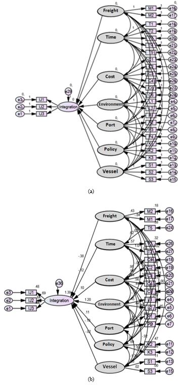Figure 1. The initial hypothesis of the SEM structural model (a), the estimation results of the structural model (b)

The initial hypothesis of the structural model was that all variables (i.e. freight, time, cost, environment, port, policy, and vessel) affect network integration (Figure 1a). Then, the initial model was tested using GOF criteria. The results of the initial test of the structural model with AMOS 23.0 showed that the negative variables for network integration were freights of -0.38, time of – 0.12, policies of -0.10 and vessels of -0.02, while the positive variables were the cost of 0.10, the environment of 1.20, and port of 0.11. The GOF test showed the sig-probability = 0.003 (not fit), RMSEA = 0.108 (not fit), GFI = 0.082 (not fit), AGFI = 0.455 (not fit), CMIN/DF = 1.813 (good fit), TLI = 0842 (marginal fit) and CFI = 0.879 (marginal fit). The results of the initial estimation of the structural model are shown in Figure 1b.

The results of the test for goodness-of-fit (GOF) criteria for the overall results of the initial estimation of the structural model are shown in Figure 1b and indicate that the model was not good because the only GOF criterion that fulfills the requirements is CMIN/DF (≤ 2.00). Therefore, it is necessary to modify the model. The process of modifying a model is basically similar to repeating the processof testing and estimating the model. The purpose of the modification is to see whether the modifications can reduce the chi-square value so that the GOF standard can be fulfilled. Modifications are performed in several ways, such as changing paths between latent variables to other latent variables, connecting latent variables to other latent variables, or connecting the manifest variable to other manifest variables, until the best model is obtained.

Sig-Probability     = 0.003 RMSEA                 = 0.108 GFI                         = 0.082 AGFI                      = 0.455 CMIN/DF             = 1.813 TLI                         = 0.842 CFI                         = 0.879

Modification of the structural model has been performed several times to obtain a model that has the best criteria for goodness-of-fit. From several experiments, we found a model that had the best criteria for goodness-of-fit, as shown in Figure 2. Modification of the SEM structural model (Figure 2) was carried out by changing the variable of the vessel path because it affected both network integration and freight, While the charge variable affected the variable of time. The results of the modification of the previous structural model assumed that the seven latent variables (i.e. freight, time, cost, environment, port, policy, and vessel) have a direct effect on network integration; however, changes occurred based on the modification results. Latent variables that affect directly the network integration were time, cost, environment, port, policy, and vessel, while the freight variable did not affect directly.

This modification of the structural model caused the elimination of two manifest variables, namely subsidy (K1) and terminal handling charge (C6). The provision of subsidies for Sea Tollway, Pelni, and Pioneer shipping was assumed to have no significant effect on network integration, because the function of subsidizing was to reduce transportation costs rather than to improve service networks directly. The terminal handling charge (THC) in the modification of the structural model was eliminated because of THC only being applied to the main port and import freights.

The results of the modification of the structural model in Figure 2 show that there was a change in the value of the latent variable which previously had a negative change to positive for network integration for the distribution of goods. Cost variable is 0.08, environment variable is 0.96, port variable is 0.24 and policy is 0.04, vessel is 0.08 and time is 0.02.

The modified structural model showed that the goodness-of-fit criteria fulfilled the requirements, where the Sig-Probability value = 0.061 (good fit), RMSEA = 0.077 (good fit), GFI = 1.034 (good fit), AGFI = 0.984 (good fit), CMIN/DF = 1,920 (good fit), TLI = 0.901 (marginal fit), and CFI = 0.882 (marginal fit). The comparison of results from running the initial model and modified models can be seen in Table 4.

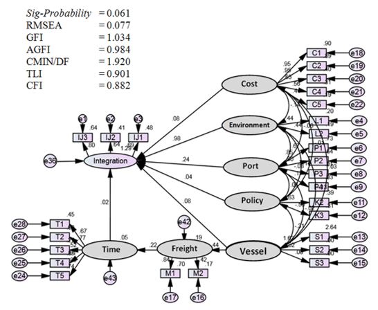Figure 2. The Best Modification Results of the Full Structural Model

Table 4. Test results on the initial structural model and modified structural model

Test Criteria	Standard cut-off value of test criteria	GOF test results		Remarks (Modified results)
		Initial model	Modified model
Sig-Probability	≥ 0.05	0.003	0.061	Good fit
RMSEA	≤ 0.08	0.108	0.077	Good fit
GFI	≥ 0.90	0.082	1.034	Good fit
AGFI	≥ 0.90	0.455	0.984	Good fit
CMIN/DF	≤ 2.00	1.813	1.920	Good fit
TLI	≥ 0.95	0.842	0.901	Marginal fit
CFI	≥ 0.95	0.879	0.882	Marginal fit

Tests on the suitability of the model indicated that the modified model was good, because sig-probability, RMSEA, GFI, AGFI, and CMIN/DF values ​​have fulfilled the predetermined requirements. Although there were variables whose values ​​were below cut off value, such as TLI and CFI (marginal fit), this model could still be accepted because the range of values ​​was still close to the cut-off value. According to Ghozali [18], if two or more of all the test criteria used have shown a good fit, it can be called as a good model.

3.4.  SEM Model Interpretation

From the results of model suitability testing, it was concluded that all variables significantly influence the integration of sea transportation networks for freight distribution in the Indonesian archipelago. The value of the test results can be seen in Table 5.

The results of the hypothesis test (Sig-Probability) in Table 5 show that all exogenous variables have an effect on an endogenous variable (network integration), thus, all hypotheses can be accepted. Estimation value shows that the time variable can be explained by sailing time indicators, loading and unloading time, berthing time, anchoring time and docking time of 87.2% while the other 12.8% is explained by indicators not contained in this paper; The cost variable can be explained by indicators of sailing costs, loading and unloading costs, inventory costs, storage costs, and container yard costs of 71.3%; Port variables can be explained by indicators of port facilities, loading and unloading equipment, pool depth of port, and distance between port of 45.8%; Vessel variables can be explained by indicators of the number of vessel operating, vessel speed and vessel capacity of 58.8%; Environmental variables can be explained by wave height indicators and weather conditions of 41.6%; Government policy variables can be explained by the shipping instruction indicator and the delivery order system of 67.2%; The freight variable does not directly affect network integration, but has a significant effect on the time of loading and unloading at the port. Same with vessel variables, in addition to influencing integration, it also has a significant effect on freight.

Table 5. Suitability Test Results of the Integration Model of the Sea Transportation Network in the Archipelago Region

Variable	Estimation	S.E	C.R	Sig-Probability	Remarks
Freight       ßVessel	0.395	0.070	11.341	0.000	Significant
Time          ßFreight	0.530	0.067	12.318	0.000	Significant
Integration ß Time	0.872	0.158	6.147	0.000	Significant
Integration ß Cost	0.713	0.064	14.233	0.000	Significant
Integration ß Environment	0.416	0.043	2.720	0.007	Significant
Integration ß Port	0.458	0.048	9.502	0.011	Significant
Integration ß Policy	0.672	0.054	16.071	0.000	Significant
Integration ßVessel	0.588	0.060	13.229	0.000	Significant

The results of the SEM model testing on the influence of each variable against the integration of sea transportation networks in the Indonesian archipelago can be interpreted as follows:

• The variable of the vessel has a significant relationship to the freight. The capacity of vessels which are currently operating tends not to be proportional to the amount of the freight carried. The average freight only reaches 40-45%, even lower. One of the reasons is the lack of interest of distributors to use Sea Tollway, Pelni, and Pioneer vessels because of the high sailing time (due to multi-port systems), in contrast to the faster private shipping liners (due to the direct shipping system) [2]. In addition, there is very little freight loaded from the destination port because it still relies on the freight of natural resources and there are no industrial products. The number of vessels operating is also not comparable with the number of islands that must be served;one vessel only serves one route. However, according to the law of the provision of PSO subsidies, the government is obliged to serve all communities fairly. Therefore, it is necessary to optimize the sea transportation service network to ensure freight distribution services in the archipelago region.
• The variable of freight has a significant relationship with time, especially sailing time, loading and unloading time, and berthing time. The sailing time is determined by the distance between the port and the speed of the vessel. In addition, it is also indirectly affected by the amount of freight. The age of the vessel used is mostly >20 years old. With the problem of age and the amount of freight, the speed of the vessel will not be maximized, so the sailing time will be longer. Berthing time at the port is the accumulation of loading and unloading time and berthing time for other activities, such as filling fuel and water. The amount of freight causes a high loading and unloading time due to the limited loading and unloading equipment at the port. Nowadays, the loading and unloading process still relies on vessel cranes, while the general freight loads of Pioneer vessels still use loading and unloading labor.
• The variable of time has a significant relationship to network integration. The main constraints of network integration are time (i.e. sailing time, loading and unloading time, berthing time, anchoring time, and docking time) [4,6,8]. Long sailing time is caused by the distance between the ports that are far away, also due to weather and wave conditions that occur in the western season [29]. Pioneer vessels sized of 500 DWT are often not allowed to sail because of the weather conditions and high waves up to 3-5 meters. The loading and unloading process at the port is considered to be ineffective because of the lack of loading and unloading equipment and still relying on labor. This condition also resulted in long berthing time at the port and high berth occupancy ratio (BOR). In certain periods, the vessel must be docked to guarantee marine reliability within 1-3 months depending on the condition of the vessel. With a limited number of vessels, the time used for the docking process will reduce distribution service performance.
• The variable of cost has a significant relationship to network integration. This is related to the economic level of each route. The chosen route must minimize distribution costs. The distribution network system in Indonesia is considered not efficient [1]. Although the distance is close, the distribution costs are not necessarily cheap, and vice versa. This condition is caused by different port costs [6]. The government, through PSO subsidies, has minimized transport costs (sailing costs), but the costs of loading, warehousing, stacking and inventory costs are still borne by the freight owner. The tendency of distributors is to choose routes that are low in cost, and they tend to ignore the long distribution time.
• Environmental variables (weather and waves) have a significant relationship to network integration. The routes of Pioneer vessels have a risk of weather conditions and high waves. The higher waves on each route, will increase the potential for accident risk [11]. Forty-eight routes of Pioneer vessels exist in eastern Indonesia, most of which are on the region that has high waves (3 to 5 meters), thus it is quite vulnerable in terms of shipping safety, especially in the west wind season.
• The variable of the port has a significant relationship to network integration. Optimizing the operation of port facilities and the productivity of loading and unloading equipment are directly related to service time. Therefore, the operational performance of port facilities must be maximized so that the time used can be minimized [7]. The operation of port facilities is represented by berth occupancy ratio (BOR), shed occupancy ratio (SOR) and yard occupancy ratio (YOR), while the productivity of loading and unloading equipment is represented by the productivity of container gantry cranes, mobile cranes, forklifts, vessel cranes, and labor. The depth of the port pond is related to the ability of the vessels to dock. Nowadays, several ports have a large demand, but the depth of the pond is not sufficient, such as for a Sea Tollway vessel with a draft of ≥ 5.5 meters, so that it can only be used by Pioneer vessels. Furthermore, network integration will be better if the service distance between ports is not too far away. Current conditions show that the distance between the ports served is classified as a long-distance track (i.e. Sea Tollway and Pelni with an average of 300-1000 sea miles, Pioneer with an average of 50-200 sea miles) thus, clustering is needed to minimize service distance.
• The variable of government policy has a significant relationship to network integration. The policy of shipping instruction and the order delivery system of Sea Tollway and Pelni vessels were still perceived as a burden on the shipper (freight owner) in the process of ordering freight space on the vessels. Nowadays, there is still a monopoly on ordering freight space and the administrative processes require a long time. The government has tried to improve the implementation of an online information system of vessels freight space, but it has not been implemented properly.
• The variable of the vessel has a significant relationship to network integration. The government, through the provision of subsidies and the PSO, commissioned the Sea Tollway, Pelni, and Pioneer vessels to serve small islands, with or without freight, routinely. However, the number of vessels operating is still not proportional to the number of ports that must be served. On the other hand, the vessels with low freight are not profitable to ship operators (i.e. Sea Tollway, Pelni, and Pioneer). If changes are made by operating a small vessel (with small load capacity and higher speed), it will be constrained by high waves.

The magnitude of the influence of each variable on the sea transport network integration illustrates that the implementation of freight distribution services in the Indonesian archipelago must pay attention to these variables. This finding is in accordance with the real conditions, in which freight distribution is often late due to weather conditions and high waves. Pioneer vessels in the western season will be difficult to sail. In addition, policy issues related to port administration and ordering procedures of freight space, and loading systems on vessels also contribute to the long waiting times for freight at the port. Another problem is the small amount of freight and sometimes there is no freight demand at one port point.

4. Conclusions

The integration of the sea transportation network to obtain a better freight distribution system in the Indonesian arcipelago, which includes the network composed of Sea Tollway, Pelni and Pioneer shipping, is directly affected by several variables. These variables can be categorized as certain and uncertain variables. The effects of the certain variables are:

• Time variables have a significant effect on network integration. 87.2% of the time variable can be explained by indicators of sailing time, loading and unloading time, berthing time, anchoring time and docking time;
• Cost variables have a significant effect on network integration. A total of 71.3% of the cost variable can be explained by indicators of sailing costs, loading and unloading costs, inventory costs, storage costs, and container yard costs;
• Port variables have a significant effect on network integration. 45.8% of port variables can be explained by indicators of port facilities, loading and unloading equipment, pool depth of port and distance between ports;
• Vessel variables have a significant effect on network integration. 58.8% of ship variables can be explained by indicators of the number of vessel operating, vessel speed and vessel capacity;

While the uncertain variables that influence network integration are:

• Environmental variables have a significant effect on network integration. 41.6% of the environmental variables can be explained by wave height indicators and weather conditions;
• Government policy variable have a significant effect on network integration. 67.2% of government policy variables can be explained by shipping instruction indicators and delivery order systems;
• Freight variable, which is loading and unloading, basically does not directly affect network integration, but has a significant effect on the time of loading and unloading at the port.

This paper has elaborated on the important aspect of variables, and further research activities can focus on defining new mathematical models to smoothly integrate sea transportation networks. Such model is expected to be able to finally optimize the freight distribution service in Indonesia.

Acknowledgments

Thank you to the Ministry of Research, Technology and Higher Education for the doctoral dissertation research grant, in order to complete doctoral studies at the Universitas Indonesia.

1.  Sonny, I., Hadiwardoyo, S. P., Susantono, B., & Benabdelhafid, A.. “The Development of a Freight Distribution Model for Connecting Inter-Island Freight Transport”. International Journal of Technology, 5, 743-750. 2015.
2.  Humang, W. P., Hadiwardoyo, S. P. & Nahry. “The Effectiveness of Pilot Marine Transport Services for Goods Distribution in Maluku Island Group, Indonesia”. In 2017 6th IEEE International Conference on Advanced Logistics and Transport (ICALT) (pp. 165-169). IEEE. 2017. 10.1109/ICAdLT.2017.8547034
3.  Walther, L., Rizvanolli, A., Wendebourg, M., & Jahn, C. “Modeling and optimization algorithms in ship weather routing.” International Journal of e-Navigation and Maritime Economy 4: 31-45. 2016. https://doi.org/10.1016/j.enavi.2016.06.004
4.  Arnone, M., Mancini, S., & Rosa, A. “Formulating a mathematical model for container assignment optimization on an intermodal network”. Procedia-Social and Behavioral Sciences, 111, 1063-1072. 2014. https://doi.org/10.1016/j.sbspro.2014.01.141
5.  Hsu, C. I., & Hsieh, Y. P. “Direct versus terminal routing on a maritime hub-and-spoke container network”. Journal of Marine Science and Technology, 13(3), 209-217. 2005. doi: 10.6119/JMST
6. Hsu, C. I., & Hsieh, Y. P. “Routing, ship size, and sailing frequency decision-making for a maritime hub-and-spoke container network”. Mathematical and Computer Modelling, 45(7-8), 899-916. 2007. https://doi.org/10.1016/j.mcm.2006.08.012
7.  Gelareh, S., & Pisinger, D. “Fleet deployment, network design and hub location of liner shipping companies”. Transportation Research Part E: Logistics and Transportation Review, 47(6), 947-964. 2011. https://doi.org/10.1016/j.tre.2011.03.002
8. He, J., Huang, Y., & Chang, D. “Simulation-based heuristic method for container supply chain network optimization”. Advanced Engineering Informatics, 29(3), 339-354. 2015. https://doi.org/10.1016/j.aei.2014.08.001
9.  Agarwal, R., & Ergun, Ö. “Ship scheduling and network design for cargo routing in liner shipping”. Transportation Science, 42(2), 175-196. 2008. https://doi.org/10.1287/trsc.1070.0205
10.  Ye, H. Q., Yuan, X. M., & Liu, X. A “Tactical Planning Model for Liner Shipping Companies: Managing Container Flow and Ship Deployment Jointly”. School of Business, National University of Singapore. 2007
11.  Vettor, Roberto, and C. Guedes Soares. “Development of a ship weather routing system.” Ocean Engineering 123: 1-14. 2016. https://doi.org/10.1016/j.oceaneng.2016.06.035
12.  Sumalee, A., Uchida, K., & Lam, W. H. “Stochastic multi-modal transport network under demand uncertainties and adverse weather condition”. Transportation Research Part C: Emerging Technologies, 19 (2), 338-350. 2011. https://doi.org/10.1016/j.trc.2010.05.018
13.  Ülengin, F., Kabak, Ö., Önsel, Ş., Ülengin, B., & Aktaş, “A problem-structuring model for analyzing transportation–environment relationships”. European Journal of Operational Research, 200(3), 844-859. 2010. https://doi.org/10.1016/j.ejor.2009.01.023
14.  Das, T., Apu, N., Hoque, M. S., Hadiuzzaman, M., & Xu, W. “Parameters Affecting the Overall Performance of Bus Network System at Different Operating Conditions: A Structural Equation Approach”. Transportation research procedia, 25, 5059-5071. 2017. https://doi.org/10.1016/j.trpro.2017.05.206
15.  Zhou, J., Guo, Y., Dong, S., Zhao, L., & Yang, R. “Structural equation modeling for pedestrians’ perception in integrated transport hubs.” Procedia engineering 137, 817-826, 2016. https://doi.org/10.1016/j.proeng.2016.01.321
16.  Papaioannou, D., & Martinez, L. M. “The Role of Accessibility and Connectivity in Mode Choice. A Structural Equation Modeling Approach”. Transportation Research Procedia, 10, 831-839. 2015. https://doi.org/10.1016/j.trpro.2015.09.036
17.  Eboli, L., & Mazzulla, G.. “Structural equation modelling for analysing passengers’ perceptions about railway services”. Procedia-Social and Behavioral Sciences, 54, 96-106. 2012. https://doi.org/10.1016/j.sbspro.2012.09.729
18.  Ghozali, I.. “Model persamaan struktural: konsep dan aplikasi dengan program Amos 16.0”. Badan Penerbit Universitas Diponegoro. 2013.
19.  Sarwono, Y.. Pengertian dasar structural equation modeling (SEM). Ilmiah Manajemen Bisnis, 10(3). 2010
20.  Lei, P. W., & Wu, Q. “Introduction to structural equation modeling: Issues and practical considerations”. Educational Measurement: issues and practice, 26(3), 33-43. 2007. https://doi.org/10.1111/j.1745-3992.2007.00099.x
21.  Vasconcelos, Adriano D., Carlos D. Nassi, and Luiz AS Lopes. “The uncapacitated hub location problem in networks under decentralized management.” Computers & Operations Research 38.12: 1656-1666. 2011. https://doi.org/10.1016/j.cor.2011.03.004
22.  Gelareh, S., Maculan, N., Mahey, P., & Monemi, R. N. “Hub-and-spoke network design and fleet deployment for string planning of liner shipping”. Applied Mathematical Modelling, 37(5), 3307-3321. 2013. https://doi.org/10.1016/j.apm.2012.07.017
23.  Hao, C., & Yue, Y. “Optimization on combination of transport routes and modes on dynamic programming for a container multimodal transport system”. Procedia engineering, 137, 382-390. 2016. https://doi.org/10.1016/j.proeng.2016.01.272
24.  Nikolaou, Michael. “Optimizing the logistics of compressed natural gas transportation by marine vessels.” Journal of Natural Gas Science and Engineering 2.1: 1-20. 2010. https://doi.org/10.1016/j.jngse.2010.02.001
25.  Pedersen, M. B., Crainic, T. G., & Madsen, O. B.. “Models and tabu search metaheuristics for service network design with asset-balance requirements”. Transportation Science, 43(2), 158-177. 2009. https://doi.org/10.1287/trsc.1080.0234
26.  Nahry, “Pengembangan Model Optimasi Sistem Distribusi Komoditsa Untuk Meningkatkan Efisiensi Sistem distribusi BUMN-PSO”, Ph.D Thesis, Universitas Indonesia. 2010.
27. Meng, Q., Wang, T., & Wang, S. “Short-term liner ship fleet planning with container transshipment and uncertain container shipment demand”. European Journal of Operational Research, 223(1), 96-105. 2012. https://doi.org/10.1016/j.ejor.2012.06.025
28.  Güner, A. R., Murat, A., & Chinnam, R. B. “Dynamic routing for milk-run tours with time windows in stochastic time-dependent networks”. Transportation Research Part E: Logistics and Transportation Review, 97, 251-267. 2017. https://doi.org/10.1016/j.tre.2016.10.014
29.  Rutz, W. O., & Coull, J. R. “Inter-island passenger shipping in Indonesia: development of the system: Present characteristics and future requirements”. Journal of Transport Geography, 4(4), 275-286. 1996. https://doi.org/10.1016/S0966-6923(96)00028-2

(Click Here)

(Click Here)