1. Introduction

The problem of describing the interaction or influence between stochastic processes has received little scrutiny in the current literature, despite its growing importance. Solving this complex problem has large implications for density estimation and knowledge discovery. In particular, for making predictions about later aspects of the process, or even for learning how processes influence each other.

Usually, the individual structure of each stochastic process is ignored and all are merged into one big process which is modelled by some probabilistic temporal model. This approach undermines the explanatory importance of the relations between these processes. [1] has explored the problems with this approach. The core of the issue mentioned by [1], is that we lose the underlying structure of the relationships between the processes which is essential to learn how one process influences another.

In this paper, we provide a complete method for learning the dynamic influence network between processes. This paper also explores the case when we are learning the influence relationship between partially observable processes. This is a significantly harder problem since the likelihood of the temporal model to the data has multiple optima which is induced from the missing samples [1]. Unfortunately, given that learning parameters from missing data is also a NP-hard problem, heuristic approaches are then needed to solve for a suitable local optimum of the likelihood function of the parameters to the data [1].

We assess this problem by providing an algorithm to learn the influence relations between partially observable stochastic processes by building on the language of probabilistic graphical modelling. In particular, we consider structure learning which searches for an appropriate structure by using scoring metrics and provide evidence for the effectiveness of our approach over the standard benchmarks selected. We notice that our derived penalty-based score paired with a greedy structure search outperforms using a random structure or a tree structure built using the maximum weighted spanning tree algorithm.

The application of this research is broad. Influence networks for stochastic processes can capture the complex relationships of how processes impact others. For example, we can learn the influence of traffic in a network of roads to determine how the traffic condition of a road congestion will impact on another road. In educational data-mining we may want to determine the influence of participants in a lecture environment to encourage student success. We may wish to learn the influence between an IoT network [1, 2]; influence in music [3]; or influence between the skills of learners or their attrition [4, 5].

An overview of the proposed algorithm in this paper is given by the below instructions. This algorithm is expanded on later in the paper.

• The stochastic processes are given as input.
• The parameters for a dynamic Bayesian network is learned for each of the stochastic processes (temporal structure remains static – time invariant and Markov).
• A structure is imposed between the dynamic Bayesian networks (using a relation function called an assemble). This gives us a dynamic influence network (DIN). The parameters for the DIN are relearned.
• The structure score for the DIN is computed.
• A structure search algorithm is initiated to find a DIN structure which is has an optimal likelihood to the observable

data;

• The optimal DIN is output.

The following contributions is made by this paper:

• The concept of dynamic influence networks (DINs) representing the influence (relationships) between partially observable stochastic processes.
• The derivation of a dynamic Bayesian information criterion (d-BIC score) for DINs.
• The concept of a structural assemble which is able to relate dynamic Bayesian networks.
• The greedy structure learning procedure for learning DINs.

The following structure is used by this paper: Section 2 provides the background and related work on DINs; Section 3 defined the representation of DINs between partially observable stochastic processes; Section 3.3 derives the notion of a dynamic structure score using the notion of an assemble; Section 3.5 provides a greedy structure learning learning algorithm for learning DINs; the results and discussion is illustrated by Section 4; and lastly, Section 5 provides the conclusion of the research and suggestions on future work.

2. Related Work

Many statistical procedures have been used to identify influence between variables [6]–[9]. These statistical procedures have been extended to the temporal environment to learn relationships the between processes (variables over time). A significant contribution is the use of dynamic Bayesian networks which is defined as a set of parameters and conditional independence assumptions which together make up an acyclic structure between variables defined using factors [10, 11]. The values in these factors are referred to as the parameters, and the list of conditional independence assumptions between variables are referred to as the structure of the dynamic Bayesian network.

Learning the independence assertions of a dynamic Bayesian network can be used to make conditional independence inferences over time (density estimation) or to simply learn the relationships between variables (knowledge discovery) [12]–[15]. On the one hand, a sparse graph structure may have more generalisability for density estimation, and on the other hand having a more dense graph can reveal unknown relationships for knowledge discovery. Care must be taken when considering for what purpose is the network required (more on this in the discussion) [11].

A successful approach to structure learning is using score-based structure learning [11, 16]. In score-based structure learning we develop a set of hypothesis structures which are evaluated using a score-based function that computes the likelihood of the data to the hypothesised structure. The likelihood is usually expressed as the information gain (mutual information) of the structure and parameters of the distribution to the data.

A search algorithm is then performed to identify the highest (possible) structure based on the structure score [17]–[20]. Viewing this problem as an optimisation problem allows us to adopt the already established literature on search methods in this super-exponential space to find the optimal structure given the data [21]–[24].

The structure of this section is as follows. In subsection 2.1 we introduce the well established BIC score which offers a way to trade-off the fit to data vs model complexity (the amount of independence assumptions between variables in the data). Finally, in subsection 2.2 we introduce a greedy search method to find the an optimal graph structure.

2.1. The BIC score

The BIC score models the structural fit to data verses the complexity of the conditional independence assumptions between variables, that is, the amount of independence assumptions made on the structure [25]. This makes it a popular choice for structure learning methods since the model complexity has a direct impact on the performance of inference tasks. This is because the amount of conditional independence assumptions on a particular variable increases the factor size of that variable exponentially. The mathematical expression of the BIC score comprises of two terms: the first term models the fit to data; and the second term penalises the fit to data based on the complexity of the structure considered. The complete BIC score is as follows:

log M score_BIC = `(θˆ_G : D) − DIM[G],

2

where the count of instances is denoted by M and the count of independent parameters is denoted by DIM[G] in the Bayesian network.

The intuition of the Bayesian score is that as the amount of samples increase (ie. M) the score is willing to consider more complicated structures if enough evidence (samples, ie. M) is considered [26, 27]. The BIC core is particularly effective since the likelihood score (one without a penalty to complexity) will always prefer the most complicated network. However, the most complex networks also impose the risk of fragmentation, which is the exponential increase to the size of the factors caused by the increase of the in-degree of a variable. Penalty-based structure scores allows us to explore the opportunity to adopt more complicated structures if there is enough justification that the likelihood of the structure and parameters to the data is high-enough to compromise on the models speed to perform inference tasks caused by fragmentation.

There has been much contributions in the literature on the properties of the BIC score [25, 28, 29]. Key constitutions include a proof the it is consistent and is score equivalent which are necessary for efficient search procedures [30]–[32].

2.2. Learning General Graph-structured Networks

Since the search space for the optimal Bayesian structure is superexponential, the difficulty of learning a graph structure for a Bayesian network is NP-hard. More specifically, for any d ≥ 2, the problem of finding a structure with a maximum score with d parents is NP-hard [21]–[24]. See [33, 34] for a detailed proof.

Despite this, there have been many contributions to learning an optimal structure. A key contribution is using heuristic search procedure to find an optimal acyclic graph structure [35]. These heuristic search procedures make use of search operators (changes to the graph structure) and a search algorithm (e.g. greedy search, best first search or simulated annealing) [36]. The intuition of this approach is find an optimal acyclic structure by gradually improving the choice of the structure using the search operators [37]–[41].

3. Dynamic Influence Networks

We present the following algorithm to learn dynamic influence networks between a set of partially observable processes:

• Our stochastic processes are given as a set of partially observed data. This is the input.
• From this data, we learn a dynamic Bayesian network for each partially observable stochastic processes. Expectation maximisation is used to learn the latent variables.
• Build a network with the set of independence assumptions and relearn the parameters for that model.
• Perform expectation maximisation once again to relearn the latent parameters of the resulting network.
• Evaluate the resulting dynamic influence network using a scoring function and structural assemble.
• Determine if convergence has occurred or if we exceed the threshold for convergence.
• Apply the structural operator to the model and reevaluate the dynamic influence network using a structure score. Repeat steps (iii – vii) until the structure score can not be improved or a threshold is reached.
• Output the resulting network.

Figure 1 provides a flowchart of our method to learn dynamic influence networks between partially observable processes.

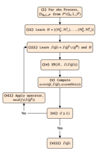
Figure 1: A flowchart of our method to learn dynamic influence networks between partially observable processes.

3.1. Assumptions

There are various assumptions we need to make about our dynamic influence network (DIN). For the below definitions, we denote ^B(_i^t) to be a shorthand for a Bayesian network B_i at time-point t.

Time Granularity Assumption We select a time-granularity, denoted 4, to split observable data into temporal time-slices at different intervals. We use the notation t4 to represent the influence state with t time-slices.

The Markov Assumption    We also adopted the Markov assumptions between consecutive states.

Definition 1 The Markov assumption is satisfied for a DIN over the template Bayesian networks, B = {B₁,…, B_R}, if for all t ≥ 0,

(B(t+1) ⊥⊥ B(0:(t−1)) | B(t)).

The Time-Invariance Finally, we assume that the unrolled template structure of the DIN (which persists through time) does not change.

3.2. Dynamic Influence Networks

Given the assumptions above we define the dynamic influence network as follows:

Definition 2 A dynamic influence network, denoted as DIN, is a couple hI₀,I_→i, where I₀ is an influence network over the set of Bayesian networks, B⁽⁰⁾ = {B₁,…, B_R}, representing the starting distribution and I_→ is a 2-time-slice influence network for the rest of the influence distribution (P(B⁰ | B_I) = ^QR_i=1 P(B⁰_i | Pa_B⁰i )). For any specified time-span T ≥ 0, the joint distribution over B^(0:T) is defined as an unrolled influence network, where, for any i = 1,…,n: the structure and conditional probability assumptions between variables of ^B(0)_i are the same as those for B_i in I₀; and the structure and conditional probability assumptions between variables of0 ^B(_i^t) for t > 0 are the same as those for B_i in I_→.

3.3. The Structure Score

In this paper we adapt the celebrated Bayesian information criterion

(BIC) to a dynamic Bayesian information criterion (d-BIC) for our dynamic influence networks. The d-BIC score make the same tradeoff between model complexity and fit to the data, only the d-BIC can be applied to dynamic networks. The d-BIC score is as follows:

                                              K        T         N

                                                       XXX hH0k,H→k i(t)                            G

scoreBIC(H0 : D) = M               (      (      (IPˆ(Xi                              ;Pa hH⁰k,H→k i(t) )))

                                             k=1     t=1     i=1                                                 ^X_i

log M

−     DIM[G], c

where the amount of samples is given by M; the amount of dependency models is given by K; the amount of time-slices is given by T for any dependency model; the amount of variables in each timeslice is given by N; I_Pˆ denotes the information gain in terms of the empirical distribution; and DIM[G] is the amount of independent parameters in the entire DIN.

The d-BIC score is designed to exchange the complexity of the dynamic influence network, ^log _c^M DIM[G], for the fit to the data, D. As the amount of samples increases, the information gain term grows linearly, and the model complexity part logarithmically grows. The intuition of the d-BIC score is that we will be willing to consider more complicated structures, if we have more data that justifies the need for a more complex model (i.e. more conditional independence assumptions).

3.4. Structure Assembles

Choosing the set of parent variables in a DIN establishes the notion of a structural assemble. A structural assemble is a template which relates temporal models. The structural assemble defines the parent sets for variables to construct an dynamic influence network. More sepcifically, the assemble relation is defined as follows:

Definition 3 Consider a family of dynamic Bayesian networks (D), where hD⁰₀, D⁰_→i represents the child with the parent set ^PaG_hD00_,D0→_i = {hD¹₀, D¹_→i,…, hD^k₀, D^k_→i}. Further assume that I(hD₀^j, D_→^j i) is the same for all j = 0,…,k. Then the delayed dynamic influence network, denoted by hA₀, A_→i, will satisfy all the independence assumptions in I , Dⁱ_→i) ∀ i = 0,…,k. In addition, ∀ j and ∀ t, hA₀, A_→i^(t) also satisfies the following independence assumptions for each hidden or latent variable denoted L_i and some t > α ∈ Z⁺:

∀ L_ihD0₀,D0→i(t): (L_ihD0₀,D0→i(t) ⊥⊥

                                                              hDk,Dk i(t)          hDk,Dk i(t)−1

             NonDescendants _hD00_,D0_→i(t) |L_i    0     →       , L_i     0     →             ,…,

L_i

L_ihDk0,Dk→i(t)−α , Pah_LD_i 00,D0→i(t)).

The assemble above an expressive representation to capture influence relationships that persist through time between temporal models. However, the choice of α is important since choosing a large α will render many dependencies on variables cause a fragmentation bottleneck, and therefore a larger computational burden for learning and inference tasks.

3.5. Structure Search

At this point we have the following well-defined optimisation problem:

1. A training set D_hI0,I→iG = {D_hD10,_D1_→i,…, D_hD0k,_Dk_→i}, where D_hDi0,_Di_→i = {ξ₁,…,ξ_M} is a set of M instances from underlying ground-truth DBN hDⁱ₀, Dⁱ_→i;
2. a structure score: score(hI₀,I_→i : D_hI_0,I_→iG);
3. and, finally, we have an array of L distinct candidate structures, G = {G¹,…, G^L}, where each structure G^l represents a unique list of condition independence assertions I(G) = I(G^I ∪ G^B).

Our objective of this optimisation problem is output the DIN which produces the maximum score. We present the following influence structure search algorithm in Algorithm 1, where S =

{S¹_→,…, S_→^P } represents the set of stochastic processes; assemble, is the option of the parameters for an assemble relation; and score, the selected scoring function used for the search procedure.

Algorithm 1: Influence structure search

Input: S = {S¹_→,…, S_→^P },assemble, score

Output: G_i

For each process we learn a temporal model

(H = {hD¹₀, D¹_→i, …, hD₀^P, D_→^P i);

Using the models in H we generate a search space (ie.

G = {G₁,…, G_n});

Find the structure G_i which produces the highest score

(w.r.t. assemble) in G; return G_i

The dynamic influence network, hI₀,I_→i^G, holds a distribution between a set of DBNs, denoted hD¹₀, D¹_→i ,…, hD^k₀, D^k_→i, with the conditional independence assumptions listed by I(hI₀,I_→i^G). We further assume that P^∗(hI₀,I_→i^G) is induced by another model, G^∗(hI₀,I_→i^G), we will refer to this model as the underlying groundtruth model. The model is evaluated by recovering the set of local independence assertions in G^∗(hI₀,I_→i^G), denoted I(G^∗(hI₀,I_→i^G)), by only observing D_hI0,I→iG. This structure learning procedure is referred to in this paper as greedy structure search (GESS).

3.6. Computational Complexity and Savings

The overall computational complexity of the above structure search algorithm is given by [42]. In order to allow for notable computational savings we suggest using a cache to store sufficient statistics and the of max priority queues (implemented using heaps) to arrange contending structure using their scores as keys. Random restarts and Tabu lists are also used.

4. Experimental Results

This sections presents the performance of modelling influence between partially observable stochastic processes using dynamic influence networks (DINs). We evaluate the performance of model aside several benchmarks.

The experimental setup is as follows. We constructed a groundtruth DIN which was used to sample sequential data. To simulate a partially observed process, several variables were removed from the sequential data sample. The Algorithm provided in section 3 was used to learn candidate networks. Several variations of the algorithm was also used, such as using the d-AIC score instead of the d-BIC; using prior knowledge of the ground-truth structure such as the maximum in-degree used in the generative distribution; using tree structure for sparse generalisability; a even using no structure.

More specifically, the empirical evaluation of our method was set against the following benchmarks:

1. a random DIN structure;
2. a DIN with no structure (i.e. all DBNs are mutually independent);
3. a DIN with a tree like structure (each DBN has one and only one parent DBN);
4. a structure that incorporates prior knowledge of the true structure;
5. a learned structure with the d-AIC score instead of the d-BIC score, which is the dynamic extension of the AIC score;
6. using the full knowledge of the DIN ground-truth structure.

The parameters for the ground-truth DIN distribution is summarised by Table 1.

Figure 2 illustrates a logarithmic scale plot indicating the relative entropy (also known as KL-divergence) to the ground-truth DIN over the amount of samples alongside the aforementioned benchmarks. The vertical axis represents the logarithmic scale of the relative entropy to the ground-truth generative model (Table 1) and the horizontal axis represents the amount of samples. 10 trials were run for each experiment and the mean of the result was plotted with the standard deviation as error bars (shaded regions). All of the model parameters for each experiment is provided in Table 2 for reproducibility.

In Figure 2 we record that providing no structure, a random structure, tree structures, and finally, learning with knowledge of the maximum order in-degree executes in a same way with reference to their relative entropy to the ground-truth DIN. However, knowledge about the maximum order in-degree executes better on average than the other procedures for a large amount of instances (greater than one thousand). The d-AIC and d-BIC scores execute on average better than the other learning procedures (not counting learning using the true structure). However, the d-BIC and d-AIC penalty scores execute similarly.

Figure 3 illustrates a logarithmic scale plot indicating the execution times (in milliseconds) over the amount of samples alongside the aforementioned benchmarks. The vertical axis represents the logarithmic scale of the execution time of each experiment in milliseconds and the horizontal axis represents the amount of samples. 10 trials were run for each experiment and the mean of the result was plotted with the standard deviation as error bars (shaded regions).

In Figure 3 we provide the results of the execution times for the learning procedures considered. With respect to their execution times, the d-AIC, d-BIC scores, and learning with knowledge of the ground-truth maximum in-degree yield the best run-time. Learning tree-structures, generating a random structures, using no structure, or being given the true structure can be achieved in constant time. It is also noticed that learning with the maximum in-degree from the ground truth can be done faster than using penalty score procedures, which have roughly the same execution time.

In the experimental learning scenario the three penalty-based learning procedures outperformed the benchmarks. Notably these penalty-based learning procedures provide significant improved performance than using no or a random structure for the DIN.

The results also indicate that learning a tree structure for the DIN still significantly outperformed the use of a random structure.

This result is particularly useful from a computational saving perspective as tree structures are sparse since they capture less complex dependence relations between variables. Tree structure summarise effective independence assertions and thus offer better generalisability. Another notable result from Figure 2 is that when we have fewer samples (> 250) we may be better suited to use no structure since imposing a structure with little training data weakens the inferences we can draw from the model.

5. Conclusion

In this paper we empirically demonstrated the a score-based structure learning procedure to learn a DIN to represent the influence relationships between partially observable stochastic processes. Why we would want to learn a DIN depends on what the structure will be used for.

On the one hand, if we are trying to identify the original DIN structure for knowledge discovery, then we will need to identify each of the original conditional independence assumptions of the ground-truth network. This means we will need to find the set I(G^∗(hI₀,I_→i^G)). This is not a promising task since there are many perfect maps for P^∗(hI₀,I_→i^G) that can be derived from D_hI_0,I_→iG.

Recognising I(G^∗(hI₀,I_→i^G)) from the set of structures from

G^∗(hI₀,I_→i^G) will yield the same fit to the data. Therefore iden-

Table 1: A table summarising the parameters for the ground-truth DIN distribution.

Ground-truth DIN Distribution
No. DBNs	10
Random variable values	3
No. time-slices	5
No. layers	2
No. CPDs between DBNs	15
max in-degree	2
No. Obs	5 p.t.
No. Latent	3 p.t.

Relative Entropy

RelativeEntropy

	Rand	No struc	Tree	GESS with PK            GESS with BIC			GESS with AIC	True
α	2	2	2	2		2	2	2
No. edges	–	–	–	15		–	–	15
Max in-degree	3	–	–	3		–	–	–
No. observable var	5	5	5	5		5	5	5
Dirichlet prior	5	5	5	5		5	5	5
Parameter threshold	–	–	–	–		5000	5000	–
EM iterations	20	20	20	20		20	20	20
EM accuracy (µ%,σ)					(76%,10)
Likelihood score	–	–	Yes	Yes		Yes	Yes	–
Penalty score	–	–	–	–		BIC	AIC	–
Search iterations	–	–	–	50		50	50	–
No. random restarts	–	–	–	5		5	5	–
Tabu-list length	–	–	–	10		10	10	–
α	2	2	2	2		2	2	2

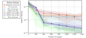
Figure 2: The relative entropy (also known as KL-divergence), to a ground truth DIN, for seven learning tasks to construct a dynamic influence network between dynamic Bayesian networks with respect to the amount of training samples.

Table 2: A table showing all of the parameters used in the structure learning methods in this paper.

Execution Time Random structure No structure Tree structures GESS with PK GESS with d-BIC GESS with d-AIC True structure

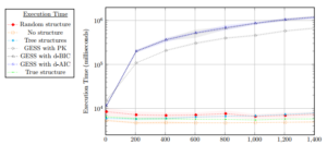
Figure 3: The execution time in milliseconds for seven learning tasks to construct a dynamic influence network between dynamic Bayesian networks with

respect to the amount of training samples. tifying the original ground-truth structure is not identifiable from D_hI0,I→iG. This is because the structures in the I-equivalent structure set all produces the same numeric likelihood (mutual information) for D_hI0,I→iG. Therefore, we should rather try to learn a set of structures that are I-equivalent to G^∗.

On the other hand, if instead we are trying to learn a DIN structure for density estimation (i.e. to draw probabilistic inferences), then we are interested in capturing the distribution P^∗(hI₀,I_→i^G). If we can successfully constructure such a distribution then we can reason about new data instances and also sample new one.

There are two implications when learning a structure or density estimation: Firstly, Although capturing more independence assertions than specified in I(G^∗(hI₀,I_→i^G)) may still allow us to capture P^∗(hI₀,I_→i^G, our selection of more independence assumptions could result in data fragmentation. Secondly, selecting too sparse structures can restrict us to never being able to learn the true distribution P^∗(hI₀,I_→i^G no matter how we change the parameters. However, often sparse DIN structures can be used to promote computational complexity savings [11].

Conflict of Interest

  The authors declare no conflict of interest.

Acknowledgement

This work is based on the research supported in part by the National Research Foundation of South Africa (Grant number: 121835).

1. R. Ajoodha, B. Rosman, “Learning the influence structure between partially observed stochastic processes using IoT sensor data,” in Workshops at the Thirty-Second AAAI Conference on Artificial Intelligence, 2018.
2. R. Ajoodha, B. Rosman, “Tracking influence between na¨ive Bayes models using score-based structure learning,” in 2017 Pattern Recognition Association of South Africa and Robotics and Mechatronics International Conference (PRASA-RobMech), 122–127, IEEE, 2017.
3. A. Anshel, D. A. Kipper, “The influence of group singing on trust and coopera- tion,” Journal of Music Therapy, 25(3), 145–155, 1988.
4. R. Ajoodha, A. Jadhav, S. Dukhan, “Forecasting Learner Attrition for Student Success at a South African University,” in In Conference of the South African Institute of Computer Scientists and Information Technologists 2020 (SAICSIT ’20), September 14-16, 2020, Cape Town, South Africa. ACM, New York, NY, USA, 10 pages., ACM, 2020, doi:https://doi.org/10.1145/3410886.3410973.
5. T. Abed, R. Ajoodha, A. Jadhav, “A Prediction Model to Improve Student Place- ment at a South African Higher Education Institution,” in 2020 International SAUPEC/RobMech/PRASA Conference, 1–6, IEEE, 2020.
6. J. Hatfield, G. J. Faunce, R. Job, “Avoiding confusion surrounding the phrase “correlation does not imply causation”,” Teaching of Psychology, 33(1), 49–51, 2006.
7. R. Opgen-Rhein, K. Strimmer, “From correlation to causation networks: a simple approximate learning algorithm and its application to high-dimensional plant gene expression data,” BMC systems biology, 1(1), 37, 2007.
8. T. Grinthal, N. Berkeley Heights, “Correlation vs. Causation,” AMERICAN SCIENTIST, 103(2), 84–84, 2015.
9. D. Commenges, A. Ge´gout-Petit, “A general dynamical statistical model with causal interpretation,” Journal of the Royal Statistical Society: Series B (Statis- tical Methodology), 71(3), 719–736, 2009.
10. M. Bunge, Causality and modern science, Routledge, 2017.
11. D. Koller, N. Friedman, Probabilistic graphical models: principles and tech- niques. (Chapter 16; 17; 18; and 19), MIT press, 2009.
12. D. Heckerman, D. Geiger, D. M. Chickering, “Learning Bayesian networks: The combination of knowledge and statistical data,” Machine learning, 20(3), 197–243, 1995.
13. A. Mohammadi, E. C. Wit, “Bayesian structure learning in sparse Gaussian graphical models,” Bayesian Analysis, 10(1), 109–138, 2015.
14. A. L. Madsen, F. Jensen, A. Salmero´n, H. Langseth, T. D. Nielsen, “A par- allel algorithm for Bayesian network structure learning from large data sets,”Knowledge-Based Systems, 117, 46–55, 2017.
15. X. Fan, C. Yuan, B. M. Malone, “Tightening Bounds for Bayesian Network Structure Learning.” in AAAI, 2439–2445, 2014.
16. C. P. d. Campos, Q. Ji, “Efficient structure learning of Bayesian networks using constraints,” Journal of Machine Learning Research, 12(Mar), 663–689, 2011.
17. S. Kok, P. Domingos, “Learning the structure of Markov logic networks,” in Proceedings of the 22nd international conference on Machine learning, 441– 448, ACM, 2005.
18. J. B. Tenenbaum, C. Kemp, T. L. Griffiths, N. D. Goodman, “How to grow a mind: Statistics, structure, and abstraction,” science, 331(6022), 1279–1285, 2011.
19. I. Tsamardinos, L. E. Brown, C. F. Aliferis, “The max-min hill-climbing Bayesian network structure learning algorithm,” Machine learning, 65(1), 31– 78, 2006.
20. S.-I. Lee, V. Ganapathi, D. Koller, “Efficient structure learning of markov net- works using l 1-regularization,” in Advances in neural Information processing systems, 817–824, 2007.
21. D. M. Chickering, D. Geiger, D. Heckerman, “Learning Bayesian networks is NP-hard,” Technical report, Technical Report MSR-TR-94-17, Microsoft Research, 1994.
22. D. M. Chickering, “Learning Bayesian networks is NP-complete,” Learning from data: Artificial intelligence and statistics V, 112, 121–130, 1996.
23. D. M. Chickering, D. Heckerman, C. Meek, “Large-sample learning of Bayesian networks is NP-hard,” Journal of Machine Learning Research, 5(Oct), 1287–1330, 2004.
24. J. Suzuki, “An Efficient Bayesian Network Structure Learning Strategy,” New Generation Computing, 35(1), 105–124, 2017.
25. G. Schwarz, et al., “Estimating the dimension of a model,” The annals of statistics, 6(2), 461–464, 1978.
26. S. Chen, P. Gopalakrishnan, “Speaker, environment and channel change de- tection and clustering via the bayesian information criterion,” in Proc. darpa broadcast news transcription and understanding workshop, volume 8, 127–132, Virginia, USA, 1998.
27. Y. Tamura, T. Sato, M. Ooe, M. Ishiguro, “A procedure for tidal analysis with a Bayesian information criterion,” Geophysical Journal International, 104(3), 507–516, 1991.
28. J. Rissanen, “Stochastic complexity,” Journal of the Royal Statistical Society. Series B (Methodological), 223–239, 1987.
29. A. Barron, J. Rissanen, B. Yu, “The minimum description length principle in coding and modeling,” IEEE Transactions on Information Theory, 44(6), 2743–2760, 1998.
30. D. Geiger, D. Heckerman, H. King, C. Meek, “Stratified exponential families: graphical models and model selection,” Annals of statistics, 505–529, 2001.
31. D. Rusakov, D. Geiger, “Asymptotic model selection for naive Bayesian net- works,” Journal of Machine Learning Research, 6(Jan), 1–35, 2005.
32. R. Settimi, J. Q. Smith, “On the geometry of Bayesian graphical models with hidden variables,” in Proceedings of the Fourteenth conference on Uncertainty in artificial intelligence, 472–479, Morgan Kaufmann Publishers Inc., 1998.
33. M. Koivisto, K. Sood, “Exact Bayesian structure discovery in Bayesian net- works,” Journal of Machine Learning Research, 5(May), 549–573, 2004.
34. T. Silander, P. Myllymaki, “A simple approach for finding the globally optimal Bayesian network structure,” arXiv preprint arXiv:1206.6875, 2012.
35. D. Chickering, D. Geiger, D. Heckerman, “Learning Bayesian networks: Search methods and experimental results,” in proceedings of fifth conference on artificial intelligence and statistics, 112–128, 1995.
36. W. Buntine, “Theory refinement on Bayesian networks,” in Proceedings of the Seventh conference on Uncertainty in Artificial Intelligence, 52–60, Morgan Kaufmann Publishers Inc., 1991.
37. A. Moore, M. S. Lee, “Cached sufficient statistics for efficient machine learning with large datasets,” Journal of Artificial Intelligence Research, 8(3), 67–91, 1998.
38. K. Deng, A. W. Moore, “Multiresolution instance-based learning,” in IJCAI, volume 95, 1233–1239, 1995.
39. A. W. Moore, “The anchors hierarchy: Using the triangle inequality to survive high dimensional data,” in Proceedings of the Sixteenth conference on Uncer- tainty in artificial intelligence, 397–405, Morgan Kaufmann Publishers Inc., 2000.
40. P. Komarek, A. W. Moore, “A Dynamic Adaptation of AD-trees for Efficient Machine Learning on Large Data Sets.” in ICML, 495–502, 2000.
41. P. Indyk, “Nearest neighbors in high-dimensional spaces,” Citeseer, 2004.
42. R. Ajoodha, Influence modelling and learning between dynamic Bayesian

(Click Here)

(Click Here)