1. Introduction

Optimisation algorithms and techniques have recently become a vast research area with the increasing availability of large datasets for DL research. Optimisation involves systematically choosing an appropriate set of values from a defined range of parameter set. These algorithms and techniques have witnessed remarkable breakthroughs in research aimed at performance improvement in applications. They are used in modelling NN to obtain better performance results by updating model parameters during the training, usually referred to as cost function in machine learning(ML). Optimisers are vital parameters when developing and deploying NN based models and help to ensure that models do not oscillate as well as preventing slow convergence [1]. Perhaps, modelling challenges have been driven research in optimisation to obtain appropriate parameters especially the assumptions made during the modelling problems as being convex functions, ill-conditioning of gradients, local minima, saddle points, plateau and flat regions, inexact, exploding gradients and cliffs, long term dependencies, theoretical limits of optimisation and poor correspondence between global and local structures [2].

To address these challenges and obtain efficient parameter learning as well as improve the performance of these learning algorithms, [3] outlined that there are three key areas to consider which include; to improve the model, to obtain better features, and lastly to improve the model inference. For large scale datasets, these improvements are necessary most importantly, to use the entire datasets for training and to obtain useful features for the learning model as well as to control the speed of learning (learning rate) of the model during the training process [4]. These large scale datasets involve massive data points and features that are used as decision variables in modelling. Some application areas that require some form of optimisation include ML, data analytics, natural language processing (NLP), among many others [5]–[6].

Cost functions have the inherent property of being convex; thus, there is always a line segment between two points on the graph of the cost function that lies on or above the chart [2]. This is achieved by reducing the difference between the predicted and actual outputs. Selecting optimal parameters for these models are difficult to achieve, with model parameters including learning rate, weights and biases, among others. The heuristic process of parameters optimisation including learning rate, weights and biases improves training stability, speed of convergence as well as a model generalisation but not currently achievable for all parameters. However, this calls for the need to review possible approaches to achieve optimal parameters. Optimisation models are used to minimise or maximise the objective function, usually referred to as the error function, cost function or loss function in literature [2]. These terms will be used interchangeably in this paper. This error function is a crucial mathematical function which depends on the model’s learnable parameters used for computing the target output from a set of inputs. The general training of NNs involves an iterative process of minimising the loss function given by

Where θ is a trainable parameter of the NN.

Conversely, as the internal parameters of the models are essential for the efficient training of the deeper architectures, which contains multiple hidden layers in their designs. The optimisation process helps the model to calculate and obtain optimal values as well as update the model parameters, thereby aiding effective learning of the features and patterns in the data. This makes the optimisation process, an essential part of model development for DL applications. This research provides a comprehensive overview of optimisation algorithms and techniques used in DL.

The remaining parts of the paper are organised as follows; Section 2 provides a brief introduction of deep learning, alongside the role of optimisers in DL research. Section 3 discusses the research method and motivation. Section 4 discusses the optimisation techniques used in DL research. Section 5 provides a brief discussion, and Section 6 presents the conclusion and future work.

2. Deep Learning

Deep learning is a sub-field of ML, where high levels of abstraction are learned from data [7]. This learning process is an iterative process that involves propagating the weights and biases of the network from input to output and vice versa. The DNNs are organized in layers, and these layers are arranged in a chain structure, with each layer being a function of the preceding layer. In this way, the overall output of the NN is obtained by computing the outputs of the successive layers from the input layer through the subsequent layers, with the output.

For a given system with n− dimensional initial inputs of X, k− layers, W− weights and b− biases ,

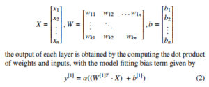
Where y¹ = first output layer, X = inputs to the model, α¹ = layer activation function (AF), W¹ = weight coefficient at layer, and b¹ = layer bias coefficients, are the parameters of the DNN. From the single layer model of equation 2, the n^th depth architecture is represented using numeric layer superscripts that shows the position of the parameters of the NN architecture, to obtain the overall output y of the very DNN as

Pictorially, we can visualise this NN, assuming five inputs, three hidden layers and an output layer is depicted in Figure 1. As the input signals are received, the hidden layers perform different transformations on the signal before propagating the signal to the output layer, where the non-linear sum of the inputs signal is obtained. This output becomes the reference output for further processing and back propagation.

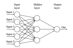
Figure 1: Neural network showing five input, three hidden and one output layer.

Conversely, the NN models consist of different architectures which are dependent on the components, arrangement, and the number of layers cascaded together, like in Figure 1. As the layers of the NN are cascaded together, more and more parameters are introduced into the network, thereby making the architecture deeper and the learning process more complicated. These models provide some distinct characteristics, mostly its scalability with increasing data and generalisation on unseen data[8].

To train these complex architectures, gradient descent is one of the most common approaches. It involves computing the minimum of a given function, by taking steps proportional to the negative of the gradient of a function at its current point [9]. During training, the inputs are forward propagated to the hidden layers and finally the output, producing a scalar cost function. This output cost is then made to flow backwards to obtain the gradient. This backward flow is known as backpropagation[10], and it involves repeated application of chain rule, across all possible paths in a NN, to obtain the gradient of each weight with respect to the corresponding output. The gradient descent would be discussed in details in the following section. Besides, as DL models depend on large amounts of data, finding the underlying patterns in the data will involve iteratively passing the data to the model until the entire examples are seen by the model, for some specified number of times, usually referred to as epochs. This entails that the models will adjust the weight and bias parameters until it attains optimal values. This adjustment process is often referred to as optimisation, and the role of these optimisation algorithms, to achieve proper learning in DNNs are outlined.

2.1. Role of Optimisers in Deep Learning

The training of DNN architectures requires the propagation of gradients to and fro the layers of the deep architectures. These gradients and their initialisation have been studied extensively alongside their propagation behaviours during the training of the learning models. Majority of these models require some optimisation to obtain the appropriate parameters. The backpropagation algorithm is one of the foremost algorithms used to compute the reverse order of computation for NNs using chain rule [10]. The backpropagation algorithm is the partial derivative of the cost function C with respect to any weights w or biases b, represented as ^∂_∂^C_w or ^∂_∂^C_b . It works by calculating the gradient of the cost function with respect to the respective weights and biases using the chain rule, while iterating backwards from the output layer, through each of the individual layers, to the inputs.

After the output is obtained by forward pass, the NN calculates the loss L, which quantifies the difference between the desired output and the actual output.The overall idea is to update the weight vectors to reduce the loss factor L. The gradient descent is used to update the weights by moving it to the opposite direction of the loss. This gradient of the loss with respect to the weights is given by

where z is the inner product, obtained by z = x^Tw and y = f(z). The update is performed in the opposite direction of the forward propagation beginning from the last layer to the first layer. This process is known as backward propagation or backpropagation. In [11], the authors highlighted that back-propagated gradients values decreases as they move from the output layers to the inputs. This causes the gradients to almost vanish at some point for very deep architectures [12], thereby requiring some optimisation to achieve an adequate learning, without dead signals. These optimisers modify the weights, biases, learning rate and other vital parameters of a model to improve the performance by reducing the losses. The numerous optimisers used to evaluate and update optimal values in these deep architectures.

3. Research Methodology and Motivation

A search of optimisers of DL was performed on the Scopus database using the keywords ”optimisers” OR ”optimizers” AND ”deep learning”, with the filter criteria outlined in Table 1. A total of 117 papers were obtained. Besides reading the titles, abstracts, and keywords, only 42 relevant articles were selected, in addition to some other articles added through cross-citation. The search results suggest that DL optimisation algorithms in literature have not been significantly explored. However, different authors have performed research on the comparison of different optimisation algorithms without a documented summary of the DL optimisers in the literature.

Nevertheless, the motivation behind this research is based on the trends observed in research publications where researchers discuss and compare the relevant DL optimisers while there is no documented research on the DL optimisers. This is evident in very recently published research where authors outlined the use of different optimisers in their research analysis including Adam, Stochastic Gradient Descent (SGD), AdaDelta, AdaGrad, RMSProp [13, 14], and many other applications outlined in the literature[15].

Table 1: Article Search Criteria

Criteria	Filter
Restriction	Title, abstract and Keywords
Language	English
Document Type	Articles
Keywords	Optimisers, Optimisation, DNN, DL, NN

Conversely, other authors considered the DNN optimisers as a tool to improve model design [16] and also to test the model performance of different applications including sign language recognition[17], optimising car crash detection [18], prediction of water leakage using Adam, RMSProp and AdaDelta [19], SGD, Adam, AdaGrad, AdaDelta, Nadam, RMSProp for bushfire prediction [20] among others. This article provides a comprehensive compilation of optimisers used in DL research. A search of the Scopus database reveals that there is considerable interest in optimisation techniques in DL with more and more researchers investigating these challenges with significant improvements since 2017, as shown in Figure 1.

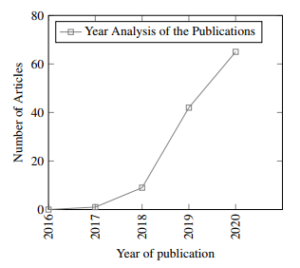
Figure 2: Scopus recent research interest for DL optimisers

However, another prominent trend in optimisation research is that it is not field-specific as authors from different fields are exploring these techniques to enhance their model performances. This is evident in Figure 3, showing the various areas of researchers investigating optimisers for DL, with computer science and engineering providing more than half of the optimisation research publications.

4. Optimisation Techniques

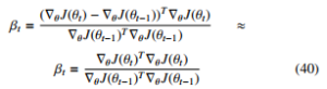
The numerous optimisation algorithms and techniques used in DNN design and applications are outlined. Due to the popularity of DL, a considerable amount of research has investigated and proposed new optimisation techniques, aimed at enhancing the model performances. These improvements outline the progress made in specific approaches and provide an entry point for discussing the current SOTA research in optimisation. Firstly, a brief outline of weight initialisation is presented since the majority of the optimisation techniques involves adjusting weights and learning rate of a model, to obtain the best features from the data. Also, the first, and second-order optimisers, the swarm intelligence optimisers, alongside parallel computing, are discussed as the other techniques of optimising DNN found in the literature results.

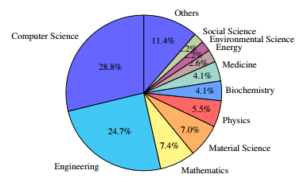
Figure 3: Scopus field of publication analysis.

4.1. Weight Initialisation

The initialisation process is a crucial optimisation approach for training DNNs. It specifies how fast the learning model converges and are used to define the starting point of a training process [21, 22], especially during the forward pass, thereby avoiding vanishing and exploding gradients. The DNNs inherently have a significant amount of parameters with a non-convex loss function response, which makes them challenging to train in real-time. To train these DNNs to achieve fast convergence while avoiding vanishing gradient problems, a careful and proper network initialisation is necessary [22, 23]. Although, it is worthy of highlighting that a proper initialisation ensures to avoid magnifying or reducing the magnitudes of a given signal exponentially [24]. While weights and biases are the key parameters to initialise, the initialisation should be able to break symmetry within the hidden units of the network.

Early weight initialisation techniques include the sparse initialisation where each unit is initialised to a constant non-zero value [25]. This approach provides more diversity in time initialised units but becomes a problem for larger Gaussian values and models with a very significant number of filters. Besides, other researchers performed initialisation differently, by initialising from Gaussian distribution with a standard deviation of 0.01, with the biases set to 1 [21], nevertheless, this technique suffers from poor convergence[24]. Other initialisation techniques include initialising with an orthonormal matrix with a carefully selected scale factor that accounts for non-linearity [26], with researchers suggesting that this technique performed better than the Gaussian distribution-based initialisation. Furthermore, the layer-sequential unit-variance(LSUV) initialisation uses the orthonormal matrices approach to pre-initialise weights of each convolution layer, with the variance of the output from the first layer normalised to 1, up to the last layer [27], in a deep CNN application.

Besides, another vital weight initialisation technique include the Xavier initialisation techniques[28], which uses a scaled uniform distribution and assumes that the activations are solely linear in all applications, thereby maintaining variance across each layer [24]. Perhaps, this is not true when the rectified activations are used in a model. This becomes a limitation for the Xavier initialisation as well as the poor convergence on very deep architectures with over thirty layers [24]. Other initialisation techniques for further exploration include the identity matrix technique, constant technique, orthogonal techniques, and variance scaling approach [26].

For proper initialisation, researchers suggest that the choice of the uniform or Gaussian distribution does not matter much but the scale of the initial distribution is a vital factor in the model optimisation [2], with the larger initial weights providing higher symmetry-breaking effect, avoidance of signal loss during forward and backwards passes, and a risk of exploding gradients. Conversely, the selection of optimal weight parameters alone cannot guarantee optimal performance especially as the behaviour of a model during the learning process is dynamic and the model parameters are not only the weights, although they are among the critical factors for the improved performance of DNNs.

4.2. Biases

The biases are vital parameters of the hidden layers of the NN. They are useful and allows for the shifting of the activation of a given NN to fit the incoming signals. It can move either left or right, thereby acting as an offset, to influence the output of the model. A crucial property of the biases is that they do not interact with the original inputs of the model as depicted in Figure 4. The initialisation of these biases is usually set to 0; however, it might be set to non-zero values in practice as researchers suggest, and that bias initialisation should not be from a random walk initialisation [29].

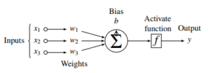
Figure 4: Typical neural network showing the positions of Weights and biases.

Conversely, initialising with high biases produces a very high output while using very low values, tends to make the signal disappear, thereby causing vanishing gradient problems. However, different architectures require different initialisation techniques; for example, the LSTM investigation have researchers suggesting to set the bias to 1, on the forget gate [30]. Another bias initialisation technique is to start with very small values, such that it would not cause massive saturation at the start especially when the rectified activations are involved [2].

Initialising the weight and bias parameters of a NN is a heuristic process and setting the bias to very small values for architectures with rectified activation is recommended while setting it to 0 for the linear activation is the standard practice. However, [2] suggest that setting biases to 0 is very compatible with the majority of the weight initialisation techniques. Perhaps, where resources permit, setting these parameters as a hyperparameter is recommended, for scales are chosen by parameter search, thereby enhancing performance. Finally, to obtain the ideal model parameters for the weights and biases involves optimisation and these optimisation techniques are presented in the subsequent sections.

4.3. First Order Optimisers (FOO)

The FOO is the dominant class of optimisers used in DL research. These models try to minimise or maximise the error function (Ex) using gradient values with respect to other parameters in the network [31, 21]. Generally, the gradient is the rate at which parameters change with time. The minimised or maximised function is usually denoted by superscript ^∗. The error function is given by [2]

Gradient descent tells when the function is increasing or decreasing at a particular point. The first order gradient produces a line tangential to a position on the error surface and is easy to compute, less time consuming and converges fast on large datasets. The variants of the first-order optimisation algorithms including batch, stochastic and mini-batch gradient descent, stochastic gradient descent with momentum as well as with warm restarts, Nesterov accelerated gradient, AdaGrad, AdaDelta, RMSProp, Adam, AdaMax, Nadam, AMSGrad, Radam and the Lookahead optimisers. These first-order algorithms are discussed in details subsequently.

4.3.1. Batch Gradient Descent (BGD)

This variant of gradient descent computes the gradient of the loss function with respect to the parameters θ for the whole training examples and update accordingly. The BGD is the default gradient descent algorithm, and it is given by

As this update is performed once, the BGD is inherently slow as well as not suitable when the entire examples cannot fit the computer memory, thereby not ideal for very DNN. The BGD does not guarantee to converge to some global minimum for convex surface errors alongside a local minimum for non-convex surfaces [32].

4.3.2. Stochastic Gradient Descent (SGD)

The SGD technique is one of the foremost approximation techniques found in the literature. It was first proposed as an approximation method of gradient optimisation by [33] and has witnessed diverse variants of optimisation to suit different applications. The stochastic gradient descent algorithm was proposed as a solution to manage the memory and speed of the BGD optimisation. The SGD solved these problems by randomly selecting the next set of examples that will update the trainable parameters, thereby improving the training speed. For a simple randomly selected examples x^(t),y^(t), the SGD is given by the relationship [34]

The advantage of SGD as outlined by [35] is that it performs better than the adaptive optimisers at very prolonged training time for effective hyperparameter tuning. However, some significant drawbacks exist for the SGD optimiser, which includes that there is no adaptive way for finding the optimal learning rate for the training process and the SGD has the gradients tending to zero at some point (saddle point), thereby making it difficult to continue alongside it’s poor convergence speed. Furthermore, other authors highlighted that the SGD does not scale well with huge datasets as well as underfitting the data for very deep architectures [36]. These drawbacks inspired further research into improving the SGD optimisation technique.

4.3.3. Mini-Batch Gradient Decent (MGD)

The MGD is an optimiser that performs an update on every batch of the training examples. The MGD offers numerous advantages which include a reduction in the variance parameter updates, thereby leading to better convergence. MGD is fully optimised for training

The limitation of MGD is that it does not guarantee excellent convergence speed as well as the difficulty of choosing the appropriate learning rate for the algorithm, which should ideally be a parameter of the dataset being considered.

4.3.4. Stochastic gradient Descent with Momentum (SGDM)

The SGDM was proposed to speed up the optimisation process of the training per dimension [37]. The process involves accelerating the process in line with the direction where the gradient points to, as well as slowing the process in the direction where the sign of the inherent gradient is changing. The classical SGDM update is given by the relationship [34]

Where v_t+1 = current velocity vector, γ = momentum term which is usually set as γ = 0.9. Alternatively, the SGDM could also be achieved by keeping track of the previous parameter updates using an exponential decay function given by

Where ρ is the decay constant controlling the previous parameter updates. The drawback for the SGDM is that the learning rate is still manually optimised, and this makes it dependent on expert judgement when trying to optimise an SGDM based model.

4.3.5. Stochastic Gradient Descent with Warm Restarts (SGDR)

The SGDR is another variant of the gradient descent optimisation that uses warm restarts instead of learning rate annealing to accelerate the training of deep neural networks. In every restart, the learning rate is initialised to a value which is scheduled to decrease. A key property of the warm restart is that the optimisation does not start from the beginning but from the parameters of the model at the last step of convergence. The decrease in learning rate is obtained using a schedule of aggressive cosine annealing given by [38]

Where η^t_min and η^t_max represents learning rate ranges and T_cur represents the number of epochs since the last restart. The T_i is the total epochs performed while i is the index of the iteration or run. The SGDR is used to deal with multi-modal functions, and these warm restart improves the rate of convergence in accelerated gradient schemes and has been successful in deep learning-based applications.

4.3.6. Nesterov Accelerated Gradient (NAG)

The Nesterov’s accelerated gradient is another first-order optimisation method that provides better convergence than gradient descent based optimisers under certain conditions [22]. The NAG optimiser was inspired by Polyak classical momentum technique of accelerating gradient descent that accumulates a velocity vector in the direction of continuous decreasing objective function [33]. Typically, given an objective function f(θ) for minimisation, the classical momentum is obtained by

Where  > 0 = learning rate, µ ∈ [0,1] = momentum coefficient and ∇ f(θ_t) = gradient at θ_t. The NAG optimiser and update rule is obtained using the relationships

The NAG computes gradient known as θ_t+1 and approximates the subsequent steps for choosing optimal step size. The NAG first moves in the direction of past accumulated gradients γv_t, computes the current gradient and updates the gradient. However, the NAG and most of the gradient-based optimisers have the same general limitation of having hand-fixed learning rate. This limitation inspires the adaptive learning-based optimisation techniques, where the learning rates may be a learnable hyperparameter. The adaptive optimisers are discussed as follows.

4.3.7. AdaGrad

The AdaGrad optimiser is an adaptive gradient algorithm proposed by [1], and it represents another vital optimiser which has adaptive parameter specific learning rates that are updated relative to the frequency of parameter updates during training. The lower learning rates implies more parameter updates during training and vice versa. The main features of the AdaGrad include fast convergence, and it considers every parameter when selecting learning rates when compared to the gradient descent techniques where one single learning rate is used for all features. This creates the flexibility of increasing or decreasing the learning rate depending on the considered feature properties.

The AdaGrad algorithm update formulation is obtained first by defining the parameters, where g_t = gradient at a time step of t, When the partial derivative of the loss function with respect to parameter θ_i, at time step t, is given by g_t,i, we can deduce the following update relationships for AdaGrad

Where η is a global learning rate shared by all dimensions, and the denominator computes an ι₂ norm of all the past gradients on each dimensional basis. g(t,i) = the gradient of the loss function with respect to parameter θ_(i) at t time step.

Generally, AdaGrad modifies the general learning rate η at every iteration of time step t for all parameters θ_(i) based on the past computed gradients for θ(i). The main identified limitations of AdaGrad includes fixing the global learning rate to a default value, the continued drop or decaying of the learning rate throughout the learning process [39] as well as the AdaGrad not been optimised for non-convex functions [2].

4.3.8. AdaDelta

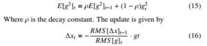
The AdaDelta is another robust adaptive learning based optimiser proposed mainly to address a significant limitation of AdaGrad by reducing the aggressiveness of AdaGrad through reduction of the optimiser learning rate. The AdaDelta optimiser uses restricted windows of past gradients, to a fixed size w, to update the learning rates rather than accumulating all the past gradients in the network [39]. Rather than storing all the inefficient previous squared gradients w, it uses the sum of exponentially decaying average of the squared gradients. At time t, the running average E[g^[1]]_t is given by

Where ∆ is the sum of the numerator term, t = time, and g = gradient. The authors enumerated the benefits of AdaDelta to include the elimination of manual fixing of learning rates, different dynamic learning rates per dimension of the parameters, less computation compared to gradient descent, robust to large gradients noise and architectures among other benefits. The author further highlighted that the hyperparameters do not require tuning, which makes the AdaDelta optimiser, a more straightforward algorithm to implement. The AdaDelta has recently been used in the design of a CNN architecture for automated image segmentation[40].

4.3.9. Root Mean Square Propagation (RMSProp)

The RMSProp is the root mean square optimisation technique which can be viewed as a modification of AdaGrad, that is optimised to perform on the non-convex setting by altering the gradient accumulation into a weighted exponential moving average. The RMSProp splits the learning rate by using an exponentially decaying average of squared gradients, and this optimiser is obtained by [2, 31]

[31] but suffers similar drawback like most of the non-adaptive optimisers as the learning rates are manually fixed or handcrafted. An advantage provided by RMSProp is that it requires less tuning compared to the SGD[35]. Besides, the RMSProp has been used in different DL architectures including to optimise the parameters of a combined deep CNN and LSTM for classifying protein structures[41] as well as the design of a new deep convolutional spiking neural network for time series classification[42].

4.3.10. Adam

Adam coined from adaptive moment estimation is another first-order gradient optimisation algorithm for stochastic objective functions based on adaptive estimates of moments of lower-order degrees. Adam is well suited for large-scale parameters and data as well as offering improved computational efficiency, improved memory requirement and invariant to the diagonal rescaling of gradients [31]. The Adam optimiser is designed to combine the properties of RMSProp and AdaGrad optimisers to obtain the first and second moments estimates which represent the mean and uncentred variance of respective gradients using

Where mˆ_t is the gradient and vˆ_t is the squared gradient and β₁, β₂ are hyperparameters that control the exponential decay rate of these moving averages, typically β₁,β₂ ∈ [0,1]. The gradient updates are estimated directly from running average of this first and second moment of a gradient to produce the update rule as

The authors outlined that the appropriate values of the parameters β₁ and β₂ are 0.9 and 0.999 respectively, while _ε= 10⁻⁸. Furthermore, they highlighted that Adam performs well in practice and compares favourably with stochastic based optimisation techniques. It also converges fast and provided a solution for the majority of the challenges faced by different optimisers which include slow convergence and vanishing gradients. The Adam optimiser has been used in the design of a new gated branch neural network for an advanced driver assistance system[43] as well as been the most used optimiser in the recent DL model developments and has been used across diverse industrial applications[44, 45].

4.3.11. AdaMax

The AdaMax optimiser is a variant of Adam with infinity norm. The velocity parameter of the algorithm scales the gradient inversely to the ι₂ norm of the previous gradients through the v_t and current gradient | g_t |² terms. The gradient is obtained by the relationship

[32]

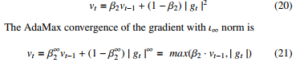
The final update rule for the AdaMax is computed as

Where u_t depends on the max operation. Default values for η = 0.002, β₁ = 0.2 and β₂ = 0.999. The AdaMax has been incorporated in the design of a deep CNN based Light Detection and Ranging (LiDAR) system application [46].

4.3.12. Nesterov  accelerated Adaptive Moment Estimation (NAdam)

The NAdam optimiser combines the properties of Adam optimiser and NAG optimiser to obtain an improved optimiser. It modifies the momentum term mˆ_t, and instead of adding the momentum term twice, the gradient is updated as gt alongside updating the parameters θ_t−1. The Nadam new update rule is written in the following form [47]

The Nadam optimiser was tested successfully on MNIST dataset, and it showed remarkable results [47].

4.3.13 AMSGrad

The AMSGrad combines the benefits of Adam and RMSProp as a moving average optimiser to guarantee convergence of learning systems. It uses lower learning rates when compared to Adam alongside incorporating slowly decaying gradients on the learning rate [48]. It also uses the maximum of past squared gradients instead of the commonly used exponential averages, to update the parameters of the optimiser where this maximum past gradient is obtained by

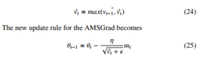
The authors outlined that the results from the testings of this AMSGrad outperformed the Adam optimiser in most cases; however, to see the practical performance of AMSGrad on more difficult datasets is still not proven. The AMSGrad has been successfully implemented for optimising the weights of deep Q-learning(DQL) used in the energy management of some hybrid electric vehicles[49].

4.3.14. Rectified Adam (RAdam)

The RAdam optimisation approach was proposed to address the large variance problem in the early stages of the adaptive learning rates by reducing the variance of the network parameters. This is achieved by rectifying the variance of the adaptive learning rate [50]. The rectified variance term is given by

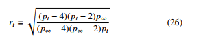
The value of p_∞ should be p_∞ ≤ 4. The authors outlined that RAdam can obtain better accuracy or an accuracy identical to Adam, with a fewer number of epochs compared to the standard Adam optimiser. The RAdam showed excellent prospects and was tested on large scale datasets to highlight the performance.

4.3.15. Lookahead

The Lookahead optimiser is another optimiser that iteratively updates two sets of weights. The unique property of the Lookahead optimiser is that it works alongside another optimiser. It updates by choosing a search direction by looking ahead at some sequence of fast weights produced by another optimiser [51]. The fast weight update rule is

Where A = optimisation algorithm, L = objective function, and d = current mini-batch training example. The authors outlined the new benefits provided by the Lookahead optimiser to include that it improves learning scalability and lowers variance with some little memory and computation cost.

4.4. Second-Order Optimisers (SOO)

The SOO uses second-order derivatives to improve model optimisation. These derivatives often referred to as Hessian matrix approximations of Hessian is useful to obtain optimal parameters during the training of NNs. These second-order models are inherently faster when the second-order derivative is known but are always costly and slower to compute in terms of memory and time. Some of the different SOO techniques used in DL are discussed in the following sections.

4.4.1. Newton’s Method

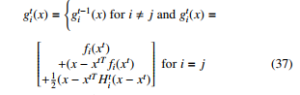
This is a second-order optimisation technique that uses secondorder Taylor series expansion to approximate J(θ) near some point θ₀ while ignoring the higher-order derivatives. The approximation relationship gives Newton’s method optimisation as

Where H is the Hessian of J with respect to θ computed at θ₀. The update rule is obtained by solving the critical point of this function given by

From the update rule, it is evident that Newton’s method involves two stages which includes computing the inverse Hessian and secondly, updating the other parameters accordingly using the iteratively computed inverse Hessian. However, this method can only work when the Hessian is positive, and this is not the case for DNNs that have built-in non-convex objective functions with saddle points, that Newton’s method cannot manage effectively without modification. A modification of Newton’s method to include a regularisation term on the Hessian is a possible solution [2]. This is achieved by adding a constant along the diagonal of the Hessian thereby changing the update rule to

This strategy works well as long as the negative eigenvalues of the Hessian remain very close to zero. Some authors have pointed out that the use of this method for training DNNs imposes a huge computational burden. By implication, it possible to train networks with a small number of parameters in practical case using Newton’s method [2], but limited in deep learning application.

4.4.2. Quasi-Newton’s Methods (QNM)

The QNM is another second-order optimisation technique used in nonlinear programming applications where Newton’s method of optimisation is difficult to use due to implementation timing constraints. They are used to find the global minimum of twice differentiable functions. The QNM requires only the gradient of the objective function to be computed during each iteration. The method is computationally cheaper and faster than the original Newton’s method approach as it does not require the computation of the inverse Hessian as well as solving systems of linear equations. The Broyden-Fletcher-Goldfarb-Shannon (BFGS) algorithm is one of the popular QNM optimisation algorithms that approximate Newton’s update rule as [2]

Where H is the Hessian of J with respect to θ computed at θ₀. The BFGS algorithm approximates the inverse of a matrix M_t, and once the inverse Hessian is updated, the direction of the descent ρ_t is determined by the relationship

A line search in the direction of the descent is performed to determine the step size ^∗ , with the final update rule as

The need to store the Hessian matrix results makes the use of the BFGS algorithm computational expensive and unrealistic for deep learning models having millions of parameters for computation during training [2]. However, more recent research using the QNM approach has been applied successfully to train DNNs on large-scale datasets[52].

4.4.3. Sum of Functions Method

The sum of functions is another second-order optimisation approach that combines the SGD and BFGS algorithms to provide improved optimisation of DNNs [52]. The authors presented a method of minimising the sum of functions that combines the efficiency of SGD with the second-order curvature information used in QNM, thereby maintaining an independent Hessian approximation, for each contributing function in the sum, for computational traceability. This optimisation approach works with mini-batches of data, alongside the deep architectures with the approximation of the series function G^t(x), defined by the intended approximate relationship

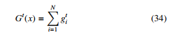
Where t = learning iteration, g^t_i(x) = quadratic approximation corresponding to f_i(x). For a vector x_t obtained by minimising the approximate objective function G^t−1(x), we have that

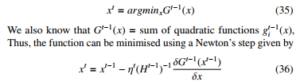
Where H^t−1 is the Hessian of G^t−1(x) and step length η^t = 1. Therefore, the update rule becomes

Where the quadratic term H_i^t is set using the BFGS algorithm. The sum of function optimiser was successfully used to train large datasets.

4.4.4. Conjugate Gradient Methods

The conjugate gradient is a Hessian free second-order optimisation technique. It avoids the use of second-order Hessian matrix in optimising gradient computation by iteratively descending conjugate directions. Though this optimisation technique is an old optimisation technique, modified versions have been successfully applied in DL research [25]. The conjugate gradient minimises the objective function with respect to parameter θ and iteratively updates the approximation of each step is given by

Where B is the Gauss-Newton matrix and δ_n represents the search direction for updating the parameter θ_n.[36] The conjugate gradient method finds a search direction that is conjugate to the previous line search direction and during the training iteration t, the new search direction takes the form [2]

Where β_t = coefficient that controls how much direction of d_t−1 that is added to the current search direction. The value of β_t can be computed using different techniques among the major ones include Polak-Ribieri and Fletcher-Reeves algorithms. The computation formula of these respective techniques is given by [2]

An important note is that for a quadratic surface, the conjugate direction ensures that the magnitude of the gradient along the previous direction does not increase. However, some researchers suggested that the second-order optimisers generally do not favour DL applications [38], and the authors highlighting the following as the reasons for that assertion about the second-order models.

• The stochastic nature of ∇ f_t(x_t).
• The ill-conditioning of parameter f.
• The presence of saddle points caused by the geometric structure of the parameter space.

This makes the first-order optimisation algorithms and techniques more useful when considering deep learning-based model parameter optimisation.

Nevertheless, another technique to improve DL model training is regularisation where dropout, dropconnect and norm regularisation techniques are used to reduce the computational cost of the model. More detailed discussions on these regularisation techniques are described in the literature[34]. Besides, other optimisation techniques include the second-order Newton’s Method, Conjugate Gradient, and Quasi-Newton’s Method (QNM), as well as the‘ parallel computing, and sum of functions. These techniques aim to improve the convergence speed of large-scale machine learning datasets. Conversely, these second-order optimisers are not always used in DL applications because of the computational burden it causes for large networks with a significant number of parameters, making them difficult for DL models having millions of parameters for computation during training [2]. However, they are gaining attention recently with researchers exploring the QNM approach to train a DNN on large-scale datasets successfully[52].

4.5. Swarm Intelligence Optimisers (SIO)

The swarm intelligence (SI) optimisers are generally computational techniques for solving distributed problems inspired by biological behavioural examples of ants, honey bees, wasps, termites, birds flocking, and many others. The SIO provides fast and reliable techniques for finding solutions on numerous real and complex problems[53]. Typical examples of SIO include ant colony optimisation, particle swarm optimisation, firefly algorithms, artificial fish swarm optimisation and many others. A very detailed survey of these dynamic SIO and algorithms can be found in this literature [54]. However, our focus lies in these optimisers that have been implemented in DL research.

4.5.1 Grey Wolf Optimiser (GWO)

The GWO is a SI optimiser that has recently been applied to DL research where the GWO was used to optimise the number of hidden layers and weights of the neural network [55]. It is proposed by [56], and it mimics the grey wolves internal leadership hierarchy in-which four key categories of wolves including alpha, beta, omega and delta was used to represent the best individual as alpha, the second-best individual as beta, the third-best individual is recorded as delta, and the remaining individuals are considered as omega. The hunting is guided by alpha, beta and delta [53]. The positions of the wolves are obtained using optimisation relationships

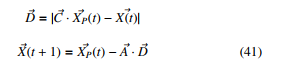
where A~ and C~ are the coefficient vector, t represents the t − th iteration, X~ is the wolf vector position and X~_P is the prey vector position. The vectors A~ and C~ is obtained by

where r~₁ and r~₂ are random vectors located in the slope of [0,1] and the value of ~a lies between 0and2.

The GWO has been recently applied in optimising flight models, especially to identify the flight state using CNNs [57] as well as modifying the hidden parameters of the SAE architecture[55]. Researchers suggest that the GWO is simple in design, fast with very high search precision, thereby making it easy to realise and implement in practical engineering applications[53]. The GWO was applied to the stacked auto-encoder (SAE) architecture for sorting different kinds of cotton [55] as well as for classifying extracted features of diabetic retinopathy dataset[58]. The GWO exploration has provided numerous improved versions, with the first being the improved Grey Wolf Optimiser (IGWO), proposed[53], as well as the multi-objective criteria version named multi-objective grey wolf optimizer (MOGWO) for DL application. The MOGWO was implemented in the long short term memory (LSTM) architecture on time series data to develop hybrid forecasting systems. Also, the use Harris hawk optimisation, which is a nature-inspired populationbased optimiser, and GWO is combined based on the mutation and hierarchy properties to produce a hybrid SI optimiser named MHHOGWO and applied in the multi-step ahead short-term forecasting of wind speeds [59].

4.5.2. Multi-swarm particle swarm optimizer and Improved Firefly Algorithm (MSPSO-ImFFA)

The MSPSO is another SI optimiser that has a modified version applied in DL research. This new adaptive MSPSO includes the improved firefly algorithms(ImFFA) that help the DNN to overcome the global and local minima as well as avoidance of premature converging during training. The MSPSO-ImFFA derivations and code can be found in the original paper[60]. The algorithms were used to train a DL backpropagation neural network (DLBPNN) for detecting and classifying lungs cancer nodules.

4.5.3. Particle Swarm Optimisers (PSO)

The PSO optimiser is another SI optimisation technique that has the ability to control the search by changing standard deviation (SD) and mean of a Gaussian distribution where the search area is linked to its SD. It uses a specific set of candidate solutions denoted by particles, that make-up the swarm population of the entire search space[61]. The improved ladder and long-tail (LLT) denoted as LLT-PSO is designed to cater for the internal setting as well as the external part of the multi-view fusion of the model. However, the model has two convolutional, and two fully-connected layers in all might not represent a typical deep architecture. The PSO has also been improved by [62] with the Adaptive Cooperative Particle Swarm Optimisation (ACPSO) proposed, which incorporates a learning automata to adaptively split the sub-population of cooperative PSO, thereby making the decision variables with strong coupling connection to enter the same sub-population. Conversely, other SI based optimisers explored for DL include the salp-swarm optimiser [63], harmony search optimiser on variational stacked autoencoders[64], whale optimisation algorithm(WOA) using bidirectional RNN [65], the Artificial Bee Colony (ABC) for optimizing hyperparameters for LSTM models, the AC-Parametric WOA (ACP-WOA) [66] for predicting biomedical images, symbiotic organisms search (SOS) algorithm [67], lion swarm optimiser(LSO) [68], and many others. Nevertheless, a comparison of the performance of these genetic algorithms shows that the GWO convergence rate is fastest compared to the Genetic Algorithm (GA), and PSO [69]. However, there is no holistic comparison of the performance of these SI optimisers found in the literature.

4.6. Parallel Computing Optimisation

Parallel computing is another optimisation approach aimed at improving the convergence speed of large-scale machine learning datasets. A popular SGD parallelised method was proposed by [70] where multi-core setting with tight coupling of the processing units ensures low latency between processors used in computing gradient updates. The parallel optimisation approach includes the synchronous and asynchronous techniques where the computation in the synchronous machines are affected by slow computers and machines on the networks causing delays [70], the asynchronous does not and it is the design model for most parallel connected devices. The parallelised SGD optimisation improves the standard SGD optimisation for application in deep learning [71]. The parallelised

The asynchronous process speeds up the training process by distributed processing with many central processing units (CPU) and graphics processing unit (GPU); however, the combination of the multiple GPU with asynchronous SGD accelerated the training process hugely [72], with the improvements in speed put at 3.2 times for four GPU’s compared to single GPU [73]. The parallelised optimisation approach has become the default approach for training very DNNs for large datasets in recent time. Conversely, the SGD has also explored the high-performance computing cluster

(HPCC) for distributed and parallelised DL applications and has been successfully implemented and tested on standard DL libraries [74].

5. Discussion

Optimisers and optimisation techniques have witnessed tremendous and advanced research results, of which there are observable trends. These trends in methods and algorithms show that there is no single existing optimiser or optimisation technique that can be used as a stand-alone optimiser for all DL research application. To achieve a holistic optimisation, the use of multiple optimisation approaches at different stages of the development and deployment of DL based models is necessary and this aligns with the no free lunch theorem that no single meta-heuristic optimisation technique can satisfy all cases and applications [75]. In a typical DL model, which involves five key stages, as shown in Figure 5. Research has shown that each of these specific stages can be optimised in one way or another. However, some of the techniques involve optimising the model design using weight initialisation, gradients, and parallel computing, as well as other model improvement techniques not discussed which include data augmentation, regularisation, dropout, batch normalisation among other methods for DL.

Figure 5: Typical deep learning model

The current application of these optimisation algorithms and techniques cuts across different industries that use neural networks to develop and deploy applications. For the stochastic gradient descent based optimisers, convergence may not be attainable when the performance of the model stops improving. A remedy to this challenges is early stopping in the case where the optimisation process is halted based on the performance of the validation set during training[76]. A proper early stopping criterion guarantees that the model training process continues as long as the network generalisation ability is improved and overfitting is avoided.

Perhaps, the current practices in the use of optimisers adopt multiple optimisation techniques where there are batch normalisation, weight and bias initialisation, data augmentation, mini-batch gradient descent, parallel computing and many other optimisation techniques involved in training a single DNN architecture. This makes most of the applications complex for development and deployment.

5.1. Application Areas

The application areas where the new optimisers are tested spans across image recognition, text classification, NLP, neural machine translation (NMT), regression-based problems. A summary table of the application areas of these optimisers are outlined. Besides, the most recent application trend is the use of SI optimisers in DL.

This optimisation approaches represent the new research direction for improving DL model performances. The summary of these optimisers alongside the test dataset are outlined in Table 2, showing the original test datasets for these optimisers.

From Table 2, it is evident that ImageNet, MNIST and CIFAR10/100 datasets rank among the most dormant datasets used in testing the new optimisation algorithms. This is as a result of the CNN architectures used for recognition applications. Although this trend is quite impressive, other datasets have also been used for NLP, and regression-based models like PT, NMT, EEG recordings and word2vec.

5.2. Model Testing Architectures

The DL architecture used in testing these novel optimisers is outlined, which include the CNN, SAE, DBN, RNN, and multi-layer neural networks (MLP), among other DNN architectures. The specific test per optimiser is presented in Table 3.

A remarkable trend in the architectures shows that major recent optimisers are tested on CNN architectures while the earliest optimisers were tested both on the MLP architectures. Also, the SI optimisers have found applications in RNN and SAE architectures, with some architectures not explicitly outlined by the authors of the original papers.

However, the use of optimisers among researchers has witnessed different researchers, selecting other datasets for testing the performance of new and ground-breaking development results. Testing these new and emerging optimisers with the same datasets or the down-sampled versions would present a reasonable and level approach to ascertain the reported results of the latest algorithm improvements. A gold standard for image recognition has been the ImageNet dataset, which one would suggest maybe the best for testing optimisers for image-based datasets alongside using the full dataset or the down-sampled versions which were used by some researchers to test their algorithm performances. A suggestion that new optimisation research and tests should use these four primary datasets including the ImageNet, MNIST and CIFAR-10/100 datasets for image-based analysis, alongside standard text and speech datasets, which will harmonise reporting of new ground-breaking results.

Conversely, comparing the SI optimisers alongside the adaptive and gradient-based optimisers is a future research mostly importantly to compare these optimisers on similar datasets. This is because most of the biological optimisers were tested on different datasets compared to the gradient-based optimisers, which were tested on mostly the four primary standard datasets.

5.3. Choosing An Optimiser

Table 2: Application areas of the various optimisation algorithms Optimiser Application Area / Datasets SGDM [21] ImageNet SGDR [38] EEG, ImageNet, CIFAR-10/100 AdaGrad [1] ImageNet, MNIST, RCVI, UCI AdaDelta [39] NLP, MNIST, Adam [31] ImageNet AMSGrad [48] MNIST, CIFAR-10 RAdam [50] NLP, ImageNet and CIFAR-10 Nadam [47] MNIST, word2vec, Penn Treebank(PT) Lookahead [51] ImageNet, CIFAR-10/100, NMT, PT GWO [56] – MOGWO [77] Electrical power and Wind speed. MSPSO-ImFFA [60] LIDC and clinical datasets LLT-PSO [61] Left ventricle and mammography Table 3: Architectures for testing the developed optimisation algorithms Optimiser CNN RNN SAE DBN MLP SGDM [21]           SGDR [38]           AdaGrad [1]   – – – – AdaDelta [39]       ∗ ∗ Adam [31]       ∗ AMSGrad [48]         ∗ RAdam [50]   ∗       Nadam [47]   ∗       Lookahead [51]   ∗       GWO [56]     ∗     MOGWO [77]   ∗       MSPSO-ImFFA [60]         ∗ LLT-PSO [61] ∗

The choice of an optimiser for a specific application is a very challenging task; however, the choice is dependent on how well the model traverses or fits on a particular task. An approach to choosing one is to consider the model architecture, the shape of the expected loss function, and picking an optimiser that can appropriately fit the data on the function. Another important consideration is the notable trade-off on the speed of convergence, training, and generalisation. These considerations were also outlined by [2], as being essential for effective optimisation. A fast convergent model that cannot generalise is not very useful, therefore finding that balance between convergence and generalisation is critical. If the training speed is the most important factor, then the Adam optimiser ranks amongst the fastest optimisers, with reasonable generalisation capability. Perhaps, if the model can train for a longer time, the SGDM can provide better convergence.

Nevertheless, the use of the SI optimisers has not been tested on the very large datasets like ImageNet and therefore, we cannot say that the SI optimisers can perform optimally on huge datasets. This limits the proposition of the most appropriate and ideal optimiser suitable for every application. An excellent approach is to test the different optimisers heuristically. This approach guarantees that the best optimiser is selected for an application.

6. Conclusion and Future Work

The DL research has witnessed a remarkable breakthrough in the development of optimisers for improving the training process of DNNs. The different optimisers used in DL research have been presented, including gradient, adaptive, hessian, and swarm-based optimisers amongst the various optimisation techniques discussed.

Besides, we outlined the different test application of these optimisers, alongside the datasets and architectures used for testing most of the discussed optimisers.

The use of compound optimisation techniques is an emerging trend in SI based optimisation research. It looks to be a future research direction while the approach might improve the gradientbased optimisation techniques. Among the investigated optimisers, first-order optimisers, especially Adam, has been the dominant optimiser, used for most DL research. It is the best performing optimiser for training very DNN architectures as validated by numerous researchers[78, 79]. However, the gradient descent-based optimisers and other adaptive optimisers have also performed remarkably in different application areas. For sparse datasets, the adaptive optimisers perform better compared to the SGD based optimisers alongside the accelerated optimisers like NAG and momentum-based optimisers. Besides, new research advances in DNN optimisation, more optimisation algorithms and techniques are being developed and with the most recent optimisers focusing on the challenges of the current optimisation algorithms.

In the future, the testing and comparing the gradient-based, adaptive, hessian and swarm optimisation techniques in DNN application will be performed to analyse and present the overall performance of these optimisers in deep learning.

[1] γE[g²]_t−1 + (1 − γ)g_t² ; θ_t−1 = θ_t − pE gη_{2t +}  · gt (17) E[g ] =

Where the appropriate values of γ = 0.9 and the learning rate η =

0.001. The RMSProp works well in stationary and online settings

1. J. Duchi, E. Hazan, Y. Singer, “Adaptive subgradient methods for online learning and stochastic optimization,” Journal of Machine Learning Research, 12(Jul), 2121–2159, 2011.
2. I. Goodfellow, Y. Bengio, A. Courville, Y. Bengio, Deep learn- ing, volume 1, MIT press Cambridge, 2016.
3. J. Turian, J. Bergstra, Y. Bengio, “Quadratic features and deep architectures for chunking,” in Proceedings of Human Lan- guage Technologies: The 2009 Annual Conference of the North American Chapter of the Association for Computational Linguistics, Companion Volume: Short Papers, 245–248, As- sociation for Computational Linguistics, 2009.
4. M. Kolbæk, Z.-H. Tan, S. H. Jensen, J. Jensen, “On loss functions for supervised monaural time-domain speech en- hancement,” IEEE/ACM Transactions on Audio, Speech, and Language Processing, 28, 825–838, 2020, doi:10.1109/TASLP. 2020.2968738.
5. A. Cassioli, A. Chiavaioli, C. Manes, M. Sciandrone, “An incremental least squares algorithm for large scale linear clas- sification,” European Journal of Operational Research, 224(3), 560–565, 2013, doi:10.1016/j.ejor.2012.09.004.
6. C.-J. Lin, R. C. Weng, S. S. Keerthi, “Trust region newton method for logistic regression,” Journal of Machine Learning Research, 9(Apr), 627–650, 2008.
7. V. Cevher, S. Becker, M. Schmidt, “Convex optimization for big data: Scalable, randomized, and parallel algorithms for big data analytics,” IEEE Signal Processing Magazine, 31(5), 32–43, 2014, doi:10.1109/MSP.2014.2329397.
8. Y. LeCun, Y. Bengio, G. Hinton, “Deep learning,” nature, 521(7553), 436, 2015, doi:10.1038/nature14539.
9. S. V. Albrecht, J. W. Crandall, S. Ramamoorthy, “Belief and truth in hypothesised behaviours,” Artificial Intelligence, 235, 63–94, 2016, doi:10.1016/j.artint.2016.02.004.
10. A. Cauchy, “Me´thode ge´ne´rale pour la re´solution des systemes d’e´quations simultane´es,” Comp. Rend. Sci. Paris, 25(1847), 536–538, 1847.
11. D. E. Rumelhart, G. E. Hinton, R. J. Williams, et al., “Learn- ing representations by back-propagating errors,” Cognitive modeling, 5(3), 1, 1988, doi:10.1038/323533a0.
12. D. Bradley, Learning in modular systems, Ph.D. thesis, The Robotics Institute, Carnegie Mellon University, 2009.
13. C. Nwankpa, W. Ijomah, A. Gachagan, S. Marshall, “Activa- tion functions: Comparison of trends in practice and research for deep learning,” CoRR, abs/1811.03378, 2018.
14. E. Okewu, P. Adewole, O. Sennaike, “Experimental compari- son of stochastic optimizers in deep learning,” in International Conference on Computational Science and Its Applications, 704–715, Springer, 2019, doi:10.1007/978-3-030-24308-1 55.
15. S. Reddy, K. T. Reddy, V. ValliKumari, “Optimization of Deep Learning Using Various Optimizers, Loss Functions and Dropout,” Int. J. Recent Technol. Eng, 7, 448–455, 2018.
16. P. Kanani, M. Padole, “Deep Learning to Detect Skin Cancer using Google Colab,” International Journal of Engineering and Advanced Technology Regular Issue, 8(6), 2176–2183, 2019, doi:10.35940/ijeat.F8587.088619.
17. J. Howard, S. Gugger, “Fastai: A layered API for deep learning,” Information, 11(2), 108, 2020, doi:10.3390/ info11020108.
18. A. Wadhawan, P. Kumar, “Deep learning-based sign language recognition system for static signs,” Neural Computing and Applications, 1–12, 2020, doi:10.1007/s00521-019-04691-y.
19. H. Robbins, S. Monro, “A stochastic approximation method,” The annals of mathematical statistics, 400–407, 1951.
20. J. Gu, Z. Wang, J. Kuen, L. Ma, A. Shahroudy, B. Shuai, T. Liu, X. Wang, G. Wang, J. Cai, et al., “Recent advances in convolutional neural networks,” Pattern Recognition, 77, 354–377, 2018, doi:10.1016/j.patcog.2017.10.013.
21. C. Garbin, X. Zhu, O. Marques, “Dropout vs. batch normal- ization: an empirical study of their impact to deep learn- ing,” Multimedia Tools and Applications, 1–39, 2020, doi: 10.1007/s11042-019-08453-9.
22. S. Sigtia, S. Dixon, “Improved music feature learning with deep neural networks,” in 2014 IEEE international confer- ence on acoustics, speech and signal processing (ICASSP), 6959–6963, IEEE, 2014, doi:10.1109/ICASSP.2014.6854949.
23. N. Qian, “On the momentum term in gradient descent learn- ing algorithms,” Neural networks, 12(1), 145–151, 1999, doi: 10.1016/S0893-6080(98)00116-6.
24. I. Loshchilov, F. Hutter, “Sgdr: Stochastic gradient descent with warm restarts,” in ICLR, 2017.
25. M. D. Zeiler, “ADADELTA: an adaptive learning rate method,” CORR, abs/1212.5701, 2012.
26. R. Hemke, C. G. Buckless, A. Tsao, B. Wang, M. Torriani, “Deep learning for automated segmentation of pelvic mus- cles, fat, and bone from CT studies for body composition assessment,” Skeletal Radiology, 49(3), 387–395, 2020, doi: 10.1007/s00256-019-03289-8.
27. S. Zhou, H. Zou, C. Liu, M. Zang, T. Liu, “Combining Deep Neural Networks for Protein Secondary Structure Prediction,” IEEE Access, 8, 84362–84370, 2020, doi:10.1109/ACCESS. 2020.2992084.
28. A. Gautam, V. Singh, “CLR-based deep convolutional spiking neural network with validation based stopping for time series classification,” Applied Intelligence, 50(3), 830–848, 2020, doi:10.1007/s10489-019-01552-y.
29. Y. Dou, Y. Fang, C. Hu, R. Zheng, F. Yan, “Gated branch neural network for mandatory lane changing suggestion at the on-ramps of highway,” IET Intelligent Transport Systems, 13(1), 48–54, 2018, doi:10.1049/iet-its.2018.5093.
30. K. Gopalakrishnan, S. K. Khaitan, A. Choudhary, A. Agrawal, “Deep convolutional neural networks with transfer learning for computer vision-based data-driven pavement distress de- tection,” Construction and Building Materials, 157, 322–330, 2017, doi:10.1016/j.conbuildmat.2017.09.110.
31. S. Das, S. Mishra, “Advanced deep learning framework for stock value prediction,” International Journal of Innovative Technology and Exploring Engineering, 8(10), 2358–2367, 2019, doi:10.35940/ijitee.B2453.0881019.
32. F. H. Nahhas, H. Z. Shafri, M. I. Sameen, B. Pradhan, S. Man- sor, “Deep learning approach for building detection using lidar–orthophoto fusion,” Journal of Sensors, 2018, 2018, doi: 10.1155/2018/7212307.
33. T. Dozat, “Incorporating nesterov momentum into adam,” in ICML, 2016.
34. S. J. Reddi, S. Kale, S. Kumar, “On the convergence of adam and beyond,” in ICLR, 2018.
35. G. Du, Y. Zou, X. Zhang, T. Liu, J. Wu, D. He, “Deep re- inforcement learning based energy management for a hybrid electric vehicle,” Energy, 117591, 2020, doi:10.1016/j.energy. 2020.117591.
36. L. Liu, H. Jiang, P. He, W. Chen, X. Liu, J. Gao, J. Han, “On the variance of the adaptive learning rate and beyond,” in ICLR, 2020.
37. M. R. Zhang, J. Lucas, G. Hinton, J. Ba, “Lookahead Opti- mizer: k steps forward, 1 step back,” CoRR, abs/1907.08610, 2019.
38. J. Sohl-Dickstein, B. Poole, S. Ganguli, “Fast large-scale op- timization by unifying stochastic gradient and quasi-Newton methods,” in ICML, 604–612, 2014.
39. J.-S. Wang, S.-X. Li, “An improved grey wolf optimizer based on differential evolution and elimination mecha- nism,” Scientific reports, 9(1), 1–21, 2019, doi:10.1038/ s41598-019-43546-3.
40. M. Mavrovouniotis, C. Li, S. Yang, “A survey of swarm intelli- gence for dynamic optimization: Algorithms and applications,” Swarm and Evolutionary Computation, 33, 1–17, 2017, doi: 10.1016/j.swevo.2016.12.005.
41. C. Ni, Z. Li, X. Zhang, X. Sun, Y. Huang, L. Zhao, T. Zhu, D. Wang, “Online Sorting of the Film on Cotton Based on Deep Learning and Hyperspectral Imaging,” IEEE Access, 8, 93028–93038, 2020, doi:10.1109/ACCESS.2020.2994913.
42. S. Mirjalili, S. M. Mirjalili, A. Lewis, “Grey wolf optimizer,” Advances in engineering software, 69, 46–61, 2014, doi: 10.1016/j.advengsoft.2013.12.007.
43. X. Chen, F. Kopsaftopoulos, Q. Wu, H. Ren, F.-K. Chang, “A self-adaptive 1D convolutional neural network for flight- state identification,” Sensors, 19(2), 275, 2019, doi:10.3390/ s19020275.
44. T. R. Gadekallu, N. Khare, S. Bhattacharya, S. Singh, P. K. R. Maddikunta, G. Srivastava, “Deep neural networks to predict diabetic retinopathy,” J. Ambient Intell. Humaniz. Comput, 2020, doi:10.1007/s12652-020-01963-7.
45. W. Fu, K. Wang, J. Tan, K. Zhang, “A composite framework coupling multiple feature selection, compound prediction mod- els and novel hybrid swarm optimizer-based synchronization optimization strategy for multi-step ahead short-term wind speed forecasting,” Energy Conversion and Management, 205, 112461, 2020, doi:10.1016/j.enconman.2019.112461.
46. H. Robbins, S. Monro, “A stochastic approximation method,” The annals of mathematical statistics, 400–407, 1951.
47. J. Gu, Z. Wang, J. Kuen, L. Ma, A. Shahroudy, B. Shuai, T. Liu, X. Wang, G. Wang, J. Cai, et al., “Recent advances in convolutional neural networks,” Pattern Recognition, 77, 354–377, 2018, doi:10.1016/j.patcog.2017.10.013.
48. C. Garbin, X. Zhu, O. Marques, “Dropout vs. batch normal- ization: an empirical study of their impact to deep learn- ing,” Multimedia Tools and Applications, 1–39, 2020, doi: 10.1007/s11042-019-08453-9.
49. S. Sigtia, S. Dixon, “Improved music feature learning with deep neural networks,” in 2014 IEEE international confer- ence on acoustics, speech and signal processing (ICASSP), 6959–6963, IEEE, 2014, doi:10.1109/ICASSP.2014.6854949.
50. N. Qian, “On the momentum term in gradient descent learn- ing algorithms,” Neural networks, 12(1), 145–151, 1999, doi: 10.1016/S0893-6080(98)00116-6.
51. I. Loshchilov, F. Hutter, “Sgdr: Stochastic gradient descent with warm restarts,” in ICLR, 2017.
52. M. D. Zeiler, “ADADELTA: an adaptive learning rate method,” CORR, abs/1212.5701, 2012.
53. R. Hemke, C. G. Buckless, A. Tsao, B. Wang, M. Torriani, “Deep learning for automated segmentation of pelvic mus- cles, fat, and bone from CT studies for body composition assessment,” Skeletal Radiology, 49(3), 387–395, 2020, doi: 10.1007/s00256-019-03289-8.
54. S. Zhou, H. Zou, C. Liu, M. Zang, T. Liu, “Combining Deep Neural Networks for Protein Secondary Structure Prediction,” IEEE Access, 8, 84362–84370, 2020, doi:10.1109/ACCESS. 2020.2992084.
55. A. Gautam, V. Singh, “CLR-based deep convolutional spiking neural network with validation based stopping for time series classification,” Applied Intelligence, 50(3), 830–848, 2020, doi:10.1007/s10489-019-01552-y.
56. Y. Dou, Y. Fang, C. Hu, R. Zheng, F. Yan, “Gated branch neural network for mandatory lane changing suggestion at the on-ramps of highway,” IET Intelligent Transport Systems, 13(1), 48–54, 2018, doi:10.1049/iet-its.2018.5093.
57. K. Gopalakrishnan, S. K. Khaitan, A. Choudhary, A. Agrawal, “Deep convolutional neural networks with transfer learning for computer vision-based data-driven pavement distress de- tection,” Construction and Building Materials, 157, 322–330, 2017, doi:10.1016/j.conbuildmat.2017.09.110.
58. S. Das, S. Mishra, “Advanced deep learning framework for stock value prediction,” International Journal of Innovative Technology and Exploring Engineering, 8(10), 2358–2367, 2019, doi:10.35940/ijitee.B2453.0881019.
59. F. H. Nahhas, H. Z. Shafri, M. I. Sameen, B. Pradhan, S. Man- sor, “Deep learning approach for building detection using lidar–orthophoto fusion,” Journal of Sensors, 2018, 2018, doi: 10.1155/2018/7212307.
60. G. Du, Y. Zou, X. Zhang, T. Liu, J. Wu, D. He, “Deep re- inforcement learning based energy management for a hybrid electric vehicle,” Energy, 117591, 2020, doi:10.1016/j.energy. 2020.117591.
61. M. Revathi, I. J. S. Jeya, S. Deepa, “Deep learning-based soft computing model for image classification application,” Soft Computing, 1–20, 2020, doi:10.1007/s00500-020-05048-7.
62. K. Lan, L. Liu, T. Li, Y. Chen, S. Fong, J. A. L. Mar- ques, R. K. Wong, R. Tang, “Multi-view convolutional neu- ral network with leader and long-tail particle swarm opti- mizer for enhancing heart disease and breast cancer detec- tion,” Neural Computing and Applications, 1–20, 2020, doi: 10.1007/s00521-020-04769-y.
63. G. Xiao, H. Liu, W. Guo, L. Wang, “A hybrid training method of convolution neural networks using adaptive co- operative particle swarm optimiser,” International Journal of Wireless and Mobile Computing, 16(1), 18–26, 2019, doi: 10.1504/IJWMC.2019.097418.
64. K. Mahmoud, M. Abdel-Nasser, E. Mustafa, Z. M Ali, “Improved Salp–Swarm Optimizer and Accurate Forecast- ing Model for Dynamic Economic Dispatch in Sustainable Power Systems,” Sustainability, 12(2), 576, 2020, doi:10.3390/ su12020576.
65. K. Chen, Z. Mao, H. Zhao, Z. Jiang, J. Zhang, “A Variational Stacked Autoencoder with Harmony Search Optimizer for Valve Train Fault Diagnosis of Diesel Engine,” Sensors, 20(1), 223, 2020, doi:10.3390/s20010223.
66. E. M. Hassib, A. I. El-Desouky, L. M. Labib, E.-S. M. El- kenawy, “WOA+ BRNN: An imbalanced big data classifi- cation framework using Whale optimization and deep neu- ral network,” soft computing, 24(8), 5573–5592, 2020, doi: 10.1007/s00500-019-03901-y.
67. A. S. Elsayad, A. I. Eldesouky, M. M. Salem, M. Badawy, “A Deep Learning H2O Framework for Emergency Predic- tion in Biomedical Big Data,” IEEE Access, 2020, doi: 10.1109/ACCESS.2020.2995790.
68. D. Prayogo, M.-Y. Cheng, Y.-W. Wu, D.-H. Tran, “Combin- ing machine learning models via adaptive ensemble weight- ing for prediction of shear capacity of reinforced-concrete deep beams,” Engineering with Computers, 1–19, 2019, doi: 10.1007/s00366-019-00753-w.
69. Z. Yang, C. Wei, “Prediction of equipment perfor- mance index based on improved chaotic lion swarm optimization–LSTM,” Soft Computing, 1–25, 2019, doi: 10.1007/s00500-019-04456-8.
70. D. D. Chakladar, S. Dey, P. P. Roy, D. P. Dogra, “EEG-based mental workload estimation using deep BLSTM-LSTM net- work and evolutionary algorithm,” Biomedical Signal Process- ing and Control, 60, 101989, 2020, doi:10.1016/j.bspc.2020. 101989.
71. M. Zinkevich, J. Langford, A. J. Smola, “Slow learners are fast,” in Advances in neural information processing systems, 2331–2339, 2009.
72. M. Zinkevich, M. Weimer, L. Li, A. J. Smola, “Parallelized stochastic gradient descent,” in Advances in neural informa- tion processing systems, 2595–2603, 2010.
73. T. Paine, H. Jin, J. Yang, Z. Lin, T. Huang, “Gpu asynchronous stochastic gradient descent to speed up neural network train- ing,” CoRR, abs/1312.6186, 2013.
74. Y. Zhuang, W.-S. Chin, Y.-C. Juan, C.-J. Lin, “A fast parallel SGD for matrix factorization in shared memory systems,” in Proceedings of the 7th ACM conference on Recommender sys- tems, 249–256, ACM, 2013, doi:10.1145/2507157.2507164.
75. R. K. Kennedy, T. M. Khoshgoftaar, F. Villanustre, T. Humphrey, “A parallel and distributed stochastic gradient descent implementation using commodity clusters,” Journal of Big Data, 6(1), 16, 2019, doi:10.1186/s40537-019-0179-2.
76. D. H. Wolpert, W. G. Macready, “No free lunch theorems for optimization,” IEEE transactions on evolutionary computation, 1(1), 67–82, 1997, doi:10.1109/4235.585893.
77. Y. Yao, L. Rosasco, A. Caponnetto, “On early stopping in gra- dient descent learning,” Constructive Approximation, 26(2), 289–315, 2007, doi:10.1007/s00365-006-0663-2.
78. D. Wei, J. Wang, K. Ni, G. Tang, “Research and Application of a Novel Hybrid Model Based on a Deep Neural Network Combined with Fuzzy Time Series for Energy Forecasting,” Energies, 12(18), 3588, 2019, doi:10.3390/en12183588.
79. M. N. Khan, M. M. Ahmed, “Trajectory-level fog detection based on in-vehicle video camera with TensorFlow deep learn- ing utilizing SHRP2 naturalistic driving data,” Accident Anal- ysis & Prevention, 142, 105521, 2020, doi:10.1016/j.aap.2020. 105521.
80. S. Remya, R. Sasikala, “Performance evaluation of optimized and adaptive neuro fuzzy inference system for predictive mod- eling in agriculture,” Computers & Electrical Engineering, 86, 106718, 2020, doi:10.1016/j.compeleceng.2020.106718.

(Click Here)

(Click Here)