1. Introduction

With the growth of communication especially using satellites and cameras, the remote sensing images was appeared with the importance of processing and dealing with this type of images (remote sensing images). One of these substantial image processing is classification which done using machine learning technology. Machine learning is one of the artificial intelligence branches that based on training computers using real data which result that computers will have good estimations as an expert human for the same type of data [1]. Deep learning is a branch of machine learning that counts on the Artificial Neural Networks (ANNs) which can be utilized in the remote sensing image classification [2]. In the recent years, which the latest satellites versions and its updated cameras with high spectral and spatial resolution are released, the very high resolution (VHR) remote sensing images are appeared. As logical results, the VHR remote sensing images have redundancy pixels that can cause an over-fitting problem through training process with using the ordinary machine learning or ordinary deep learning in classification. So it must optimize the ANNs and extract convenient features from remote sensing images as a preprocessing before training [3]. The convolution neural networks (CNNs) are derived from the ANNs who haven’t fully connected layers as the ANNs layers; it have an excited rapid advance in computer vision [4]. It is based on some blocks can enforced on images as filters and then extracting a convolution object features from the input images which solving many of computer vision problems, one of these problems is classification [5]. The need of dealing with the huge data, that be contained in the VHR remote sensing images, produced the need of specific CNNs deep networks architectures that can generate an elevated accuracy in the classification problems. So, the classic networks are appeared. Many of classic networks are mentioned by researchers in their research papers. In this paper we use three widely used classic networks as features extraction in our proposed approaches. These classic networks are; the DenseNet 196, the VGG 16, and the ResNet 50 models. There are many researchers used these networks in their researches that related to the remote sensing images classification. In [6], authors proposed a new model to improve the classification accuracy using the DenseNet model. In [7], authors built dual channel CNNs for the remote sensing images using the DenseNet as features extraction. In [8], authors built small number of convolutional kernels using dense connections to achieve large number of reusable feature maps. It was lead them to propose a convolutional network based on the DenseNet for the remote sensing images classification. In [9], authors used the VGG and the ResNet models to propose the RS-VGG classifier for classifying the remote sensing images. In [10], authors were built a combination between CNNs algorithms outputs, the VGG model is one of these algorithms, so a representation of the VHR remote sensing images understanding were established by their proposed method. In [11], authors used the remote sensing images classification to distinguish the airplanes by using the pre-trained VGG model. In [12], authors built a classifier model that classifying the high spatial resolution remote sensing images by using a fully convolution network that based on the VGG model. In [13], authors proposed the use of the ResNet model to extract the VHR remote sensing images features, then concatenated with low level features to generate a more accurate model using the SVM. In [14], authors used the ResNet to extract the 3-D features by transfer learning. They proposed a classification method for the hyper-spectral remote sensing images. In [15], authors proposed a method for classifying forest tree species using high resolution RGB color images that captured by a simple grade camera mounted on an unmanned aerial vehicle (UAV) platform. They used the ResNet in their proposed. In [16], authors proposed aircraft detection methods that based on the deep ResNet and super vector coding. In [17], authors combined edge and texture maps to propose a remote sensing image usability assessment method based on the ResNet. In [18], authors presented a comparative study that discussed the difference between the using of the SVM and the deep learning in classifying the remote sensing images. In [19], authors proposed a remote sensing image classification method that based on the SVM and sequential classifier. In [20], authors proposed a remote sensing images classifier using the genatic algorithm (GA) and the SVM.

The problem that attended by this paper is the difficulty of reaching a high accuracy assessment in the VHR remote sensing images classification models. Many researchers proposed solutions for this problem in their researches but they depend on the deep learning only or the machine learning only. Few of them are proposed hybrid classification techniques that consist of combination of the deep learning and the machine learning such as [13] and [20]. The deep learning and the machine learning combination can lead to considerable results.

The aim of this paper is to propose a combination of a classic network and the SVM to build a novel remote sensing images classifier. In this paper, the desired classic networks that combined with the SVM classifier are the DenseNet 169, The VGG16, and the ResNet 50 models. We used the ImageNet pre-trained weights with these mentioned models, transfer learning, and then extract features. These extracted features are considered as input features for the SVM classifier which trained to achieve the desired performance classification models. A comparative study is done for the use of the mentioned three convolution models as features extraction that combined with the SVM classifier, as proposed in this paper, to determine the performance of using each model. This comparison is based on calculating the overall accuracy (OA) to determine the performance of each model as a features extraction. There are two used datasets in this study; the UC Merced land use dataset and the SIRI-WHU dataset.

The rest of this paper is organized as follow. Section 2 gives the methods. The experimental results and setup are shown in section 3. Section 4 presents the conclusions followed by the most relevant references.

2. The Methods

In this section the proposed models will explained with its structures. The classic networks that used in these proposals and the SVM will illustrate in brief as a literature review, ending with how to measure the learning model performance.

2.1. The Proposed Models

The features extraction from the remote sensing images is provided an important basis in the remote sensing images analysis. So, in this paper the classic networks outputs can considered as the features that extracted from the remote sensing images. Where the train of a new model of the CNNs requires large amount of data, so in these three models, we used the ImageNet pre-trained weights, transfer learning, and then extract the desired features, then use these features as input features in training the SVM classifier. In the DenseNet 169 model, we transfer learning to the last hidden layer, before the output layer, that had 1664 neurons. Its outputs considered as the input features for the SVM classifier. In the VGG 16 model, we transfer learning to the last hidden layer, before the output layer, that had 4096 neurons. Its outputs considered as the input features for the SVM classifier. In the ResNet 50 model, we transfer learning to the last hidden layer, before the output layer, that had 2048 neurons. Its outputs considered as the input features for the SVM classifier.

2.2. The Convolution Neural Networks (CNNs)

The CNNs are possessed from the ANNs with exclusion that it is not fully connected layers [21]. The CNNs considered as the magic solution for much computer vision problems. The CNNs depend on some of filters that reduce the image height and width and increase the number of channels, then processing the output with full connected (FC) neural network layers [21, 22]. Figure 1 shows one of the CNNs model structures [22].

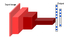
Figure 1: One of the CNNs model structures [23]

2.3. The DenseNet Model

In 2017, the DenseNets was proposed in the CVPR 2017 conference (Best Paper Award) [23]. The start point was from endeavored to construct a deeper convolution network that contains shorter connections between its layers close to the input and those close to the output, this deep convolution network can be more accurate and efficient to train. It is different from the ResNet which has skip-connections that bypass the nonlinear transformation, the DenseNet add a direct connection from any layer to any subsequent layer. So the  layer receives the feature-maps of all former layers  to  as (1) [23].

where  refers to the spectrum of the feature-map produced in the layers . Figure 2 shows the 5-layers dense block architecture. Table 1 shows the DenseNet 169 model architecture with the ImageNet pre-trained weights [23].

Table 2: The VGG 16 model architectures for ImageNet [24]
Block	Layers	Output Size	VGG 16
Input		224 224 3
Block 1	Convolution	224 224 64	3 3 conv 64, stride 1
	Convolution	224 224 64	3 3 conv 64, stride 1
	Pooling	112 112 64	2 2 max pool, stride 2
Block 2	Convolution	112 112 128	3 3 conv 128, stride 1
	Convolution	112 112 128	3 3 conv 128, stride 1
	Pooling	56 56 128	2 2 max pool, stride 2
Block 3	Convolution	56 56 256	3 3 conv 256, stride 1
	Convolution	56 56 256	3 3 conv 256, stride 1
	Convolution	56 56 256	3 3 conv 256, stride 1
	Pooling	28 28 256	2 2 max pool, stride 2
Block 4	Convolution	28 28 512	3 3 conv 512, stride 1
	Convolution	28 28 512	3 3 conv 512, stride 1
	Convolution	28 28 512	3 3 conv 512, stride 1
	Pooling	14 14 512	2 2 max pool, stride 2
Block 5	Convolution	14 14 512	3 3 conv 512, stride 1
	Convolution	14 14 512	3 3 conv 512, stride 1
	Convolution	14 14 512	3 3 conv 512, stride 1
	Pooling	7 7 512	2 2 max pool, stride 2
FC		4096
FC		4096
Output		1000, softmax

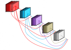
Figure 2: The 5 layers Dense block architecture [23]

2.4. The VGG Model

In 2015, the VGG network was proposed in the ICLR 2015 conference [24]. The start with inspected the effect of the convolution network depth on its accuracy with using the large-scale images. Through they rectified the deeper networks architecture using (3 3) convolution filters, they showed that an expressive growth on the prior-art configurations can be achieved by pushed the depth to 16-19 weight layers. The VGG model is a deeper convolution network that trained on the ImageNet dataset. Table 2 shows the VGG 16 model architecture with the ImageNet pre-trained weights [24].

Table 2: The VGG 16 model architectures for ImageNet [24]
Block	Layers	Output Size	VGG 16
Input		224 224 3
Block 1	Convolution	224 224 64	3 3 conv 64, stride 1
	Convolution	224 224 64	3 3 conv 64, stride 1
	Pooling	112 112 64	2 2 max pool, stride 2
Block 2	Convolution	112 112 128	3 3 conv 128, stride 1
	Convolution	112 112 128	3 3 conv 128, stride 1
	Pooling	56 56 128	2 2 max pool, stride 2
Block 3	Convolution	56 56 256	3 3 conv 256, stride 1
	Convolution	56 56 256	3 3 conv 256, stride 1
	Convolution	56 56 256	3 3 conv 256, stride 1
	Pooling	28 28 256	2 2 max pool, stride 2
Block 4	Convolution	28 28 512	3 3 conv 512, stride 1
	Convolution	28 28 512	3 3 conv 512, stride 1
	Convolution	28 28 512	3 3 conv 512, stride 1
	Pooling	14 14 512	2 2 max pool, stride 2
Block 5	Convolution	14 14 512	3 3 conv 512, stride 1
	Convolution	14 14 512	3 3 conv 512, stride 1
	Convolution	14 14 512	3 3 conv 512, stride 1
	Pooling	7 7 512	2 2 max pool, stride 2
FC		4096
FC		4096
Output		1000, softmax

The input images of this network is (224 244 3). This network consists of five convolution blocks, each block containing convolution layers and pooling layer, then ending with two FC hidden layers (each layer has 4096 neurons), then ending with the output layer with softmax activation (1000 classes) [24].

2.5. The ResNet Model

In 2016, the ResNet was proposed in the CVPR 2016 conference [25]. They concerted the degradation problem by presenting a deep residual learning framework. Instead of intuiting, each few stacked layers directly fit a desired underlying mapping. The ResNet is based on skip connections between deep layers. These skip connections can skipping one or more non-linear transformation layers. The outputs of these connections are added to the outputs of the network stacked layers as (2) [25].

where H(x) is the final block output, x is the output of the connected layer, and F(x) is the output of the stacked networks layer in the same block. Figure 3 shows the ResNet one building block and tables 3 shows the ResNet 50 model architecture for the ImageNet [25].

Table 3: the ResNet 50 model architectures for ImageNet [25]

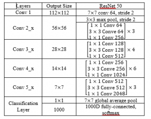
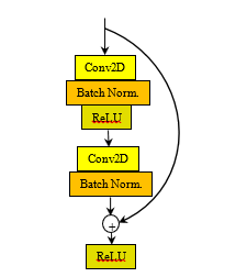
Figure 3: The ResNet building block[25]

2.6.  The Support Vector Machine (SVM)

The SVM is a machine learning algorithm can act as a classifier or regression. It is based on small sample statistic theory that establishes optimal hyper-planes from the training data. These hyper-plans separate the different classes by building margins between classes. Maximizing these margins between classes, specially the nearest classes, on both sides of hyper-planes is the target for achieving the optimal SVM classifier [26, 27]. Figure 4 shows the possible and the optimal hyper-planes in the SVM model [26, 27].

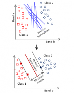
Figure 4: The possible and the optimal hyper-planes in the SVM model [26, 27]

2.7. The Performance Assessment

There are many matrices for gauge the performance of the learning models. One of them is the overall accuracy (OA). The OA is the main classification accuracy assessment [28]. It is measure the percentage ratio between the corrected estimation test data objects and all the test data objects in the used dataset. The OA is calculated using (3) [28, 29].

3. Experimental Results and Setup

This section will illustrate the experiments setup of the proposed algorithms, and then presents a comparative study for using each convolution model in our proposed. This comparison is based on calculating the OA for each model. The UC Merced land use dataset and the SIRI-WHU dataset are the used datasets. The details of these datasets will introduce in this section and then the experiments setup and results.

3.1. The UC Merced Land Use Dataset

The UC Merced Land use dataset is a collection of remote sensing images which has been prepared in 2010 by the University of California, Merced [30]. It is consists of 2100 remote sensing images divided into 21 classes with 100 images per each class. The images were manually extracted from large images from the USGS National Map Urban Area Imagery collection for various urban areas around the USA. All images in this dataset are Geo-tiff RGB images with 256 256 pixels resolution and 1 square foot (0.0929 square meters) spatial resolution [30]. Figure 5 shows image examples from the 21 classes in the UC Merced land use dataset [30].

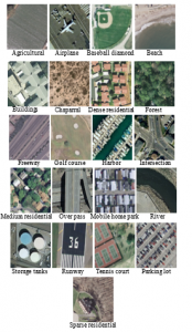
Figure 5: Image examples from the 21 classes in the UC Merced land use dataset [30]

3.2. The SIRI-WHU Dataset

The SIRI-WHU dataset is a collection of remote sensing images which the authors of [31] used this dataset in their classification problem research in 2016. This dataset consists of two versions that must complete each other. The total images in this dataset are 2400 remote sensing images divided into 12 classes with 200 images per each class. The images were extracted from Google Earth (Google inc.) and mainly cover urban areas in China. All images in this dataset are Geo-tiff RGB images with 200 200 pixels resolution and 2 square meters (21.53 square foot) spatial resolution [31]. Figure 6 shows image examples from the 12 classes in the SIRI-WHU dataset [31].

Figure 6: Image examples from the 12 classes in the SIRI-WHU dataset [31].

3.3. The Experimental Setup

All tests were performed using Google-Colab. The Google-Colab is a free cloud service hosted by Google inc. to encourage machine learning and artificial intelligence researches [32]. It is acts as a virtual machine (VM) that using 2-cores Xeon CPU with 2.3 GHz, GPU Tesla K80 with 12 GB GPU memory, 13 GB RAM, and 33GB HDD with Python 3.3.9. The maximum lifetime of this VM is 12 hours and it will be idled after 90 minutes time out [33]. Performing tests has been done by connecting to this VM online through ADSL internet line with 4Mbps communication speed. This connection was done using an Intel® coreTMi5 CPU M450 @2.4GHz with 6 GB RAM and running Windows 7 64-bit operating system. This work is limited by used the ImageNet pre-trained weights because the train of new convolution models needs a huge amount of data and more sophisticated hardware, this is unlike the lot of needed time consumed for this training process. The other limitation is that the input images shape is mustn’t less than 200 200 3 and not greater than 300 300 3 because of the limitations of the pre-trained classic networks. The preprocessing step according to each network requirements is necessary to get efficient results; it must be as done on ImageNet dataset through these models were trained and produced the ImageNet pre-trained weights. The ImageNet pre-trained weights classic networks that used in this paper have input shape (224, 224, 3) and output layer with 1000 neurons according to the ImageNet classes (1000 classes) [34, 35]. So, it must perform transfer learning as stated in section 2.1. The used datasets were divided into 80% training set and 20% testing set before training the SVM model. It is must be notice that the SVM penalty value were determined by iterations and self-intuition. To extract the convolution features, the normalization preprocessing must done before extract features using the DenseNet 169 model, then using these features as input features to train the SVM model with penalty = 1.7. Where the BGR mode convertion is the desired preprocessing before extract features using the VGG 16 and the ResNet 50 models, then using its outputs as input features to train the SVM model with penalty = 2 for the VGG 16 extracted features and penalty =20 for the ResNet 50 extracted features. Figure 7 shows the flow charts of the proposed algorithms in this paper; figure 7.a. for using the DenseNet 169 model as features extraction, figure 7.b. for using the VGG 16 model as features extraction, and figure 7.c. for using the ResNet 50 model as features extraction, and then training the SVM classifier.

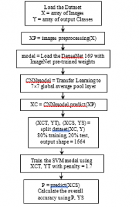
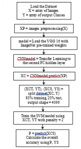
Figure 7: The flow charts of the proposed algorithms in this paper

3.4. The Experimental Results

This section presents the results of the proposed algorithms with the used datasets in this paper. Through the training process we used the training data (80% from the used dataset) and then calculate the OA using the predictions of the test data (20% from the used dataset) to assess the performance of each model. Table 4 and figure 8 show the OA for the using of each model to extract features that act as the input features to train the SVM classifier using the both datasets.

Table 4: The OA for the use of the convolution models with the SVM classifier using the both datasets
	The DenseNet-SVM	The VGG-SVM	The ResNet-SVM
The UC Merced land use Dataset	0.902	0.881	0.926
The SIRI-WHU Dataset	0.94	0.942	0.958

As shown from these results, the ResNet–SVM model had the higher OA in this study where the VGG–SVM model had the lowest OA. In the other hand the DenseNet–SVM model had higher OA than the VGG–SVM model when using the UC Merced land use dataset and had very little lower OA than the VGG–SVM when using the SIRI-WHU dataset. The use of the SIRI-WHU dataset had higher OA than the use of the UC Merced land use dataset. These results illustrated that the OA had an opposite relation with the dataset image resolution and the dataset number of classes, so the use of the SIRI-WHU dataset which has 12 classes, image resolution 200 200 pixels, and spatial resolution 2 square meters gave higher OA than the use of the UC Merced land use dataset which has 21 classes, image resolution 256 256 pixels, and spatial resolution 0.0929 square meters (1 square feet). Extracting features using the deeper convolution networks gave considerable accuracy but the connections between layers may have another influence. The VGG–SVM model, that has deeper network without any layers connections, gave a good OA so it had an efficient result. In the other hand the ResNet–SVM model, that has skip layers connections, and the DenseNet–SVM, that has full layers connections, gave higher OA but still the ResNet–SVM gave the highest OA in this comparison. If keeping in mind the penalty values that used in training the SVM classifier using the three models as features extraction, we saw that the VGG–SVM and the DenseNet–SVM had normal penalty to give its OA in this comparison, where the ResNet–SVM had a high penalty value and given the highest OA in this comparison. The ResNets are based on the skip layers connections so the layer connections can raise the classification accuracy. The DenseNets may have more connections but still the use of the ResNets has the higher OA. As a total the deeper convolution networks may give better accuracy but the deeper networks that have layers connections may give the more better accuracy. The convolution models that have skip connections can give the better OA than the convolution models that have full layers connections. A high penalty value is needed for training the SVM models when using input features that extracted from the skip connection convolution models. For the SVM classifiers, extracting features from the high resolution remote sensing images are preferred with the use of deep convolution models that have layers connections where extracting features from the low resolution remote sensing images are preferred with the use of deep convolution models that haven’t layers connections.

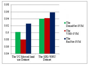
Figure 8: The OA for the use of the convolution models with the SVM classifier using the both datasets

4. Conclusions

This paper proposed remote sensing images classification approaches using the SVM classifier. The proposed approaches were based on using the deep convolution models classic networks as features extraction. The used classic networks in these approaches were the Densenet 169, the VGG 16, and the ResNet 50 models. The remote sensing images convolution features were extracted from these convolution models using the ImageNet pre-trained weights, which used as input features to train the SVM classifier. This paper also presented a comparison between the uses of the mentioned convolution models with the SVM classifier as proposed in this paper. This comparison was based on calculating the OA for using each model with the SVM classifier. There were two used datasets in this study; the UC Merced land use dataset and the SIRI-WHU dataset. This comparison illustrated that the ResNet–SVM model was more accurate than the other models that mentioned in this paper, which the OA of the DenseNet–SVM model was higher than the VGG–SVM model for using the UC Merced land use dataset and very little lower than the VGG–SVM using the SIRI-WHU dataset. The overall accuracy had an opposite relation with the remote sensing images resolution (pixel or spatial) and the number of dataset classes. For the SVM classifiers, it is preferred to use the deep networks without layers connections as features extraction with the low resolution remote sensing images where the deep networks that have layers connection are the preferred with the high resolution remote sensing images.

Conflict of Interest

The authors declare no conflict of interest.

1. M. Bowling, J. Furnkranz, T. Graepel, and R. Musick, “Machine Learning and Games”, Machine Learning, Springer, 63(3), 211-215, 2006. http://doi.org/10.1007/s10994-006-8919-x
2. K. Hwan Kim and S. June Kim, “Neural Spike Sorting Under Nearly 0-dB Signal-to-Noise Ratio Using Nonlinear Energy Operator and Artificial Neural-Network Classifier”, IEEE Transactions on Medical Engineering, 47(10), 1406-1411, 2000. http://doi.org/10.1109/10.871415
3. M. Nair S., and Bindhu J.S., “Supervised Techniques and Approaches for Satellite Image Classification”, International Journal of Computer Applications (IJCA), 134(16), 1-6, 2016. http://doi.org/10.5120/ijca2016908202
4. W. Rawat, and Z. Wang, “Deep Convolutional Neural Networks for Image Classification: A Comprehensive Review”, Neural computation, 29(9), 2352-2449, 2017. http://doi.org/10.1162/NECO_a_00990
5. A. Khalid et al., “Artificial Neural Networks Optimization and Convolution Neural Networks to Classifying Images in Remote Sensing: A Review”, in The 4th International Conference on Big Data and Internet of Things (BDIoT’19), 23-24 Oct, Rabat, Morocco, 2019. http://doi.org/10.1145/3372938.3372945
6. Y. Tao, M. Xu, Z. Lu, and Y. Zhong, “DensNet-Based Depth-Width Double Reinforced Deep Learning Neural Network for High-Resolution Remote Sensing Images Per-Pixel Classification”, Remote Sensing, 10(5), 779-805, 2018. http://doi.org/10.3390/rs10050779
7. G. Yang, B. Utsav, E. Ientilucci, Micheal Gartley, and Sildomar T. Monteiro, “Dual-Channel DenseNet for Hyperspectral Image Classification”, in IGARSS 2018 – 2018 IEEE International Geoscience and Remote Sensing Symposium, 05 Nov, Valencia, Spain, 2595-2598, 2018. http://doi.org/10.1109/IGARSS.2018.8517520
8. J. Zhang, C. Lu, X. Li, H. Kim, and J. Wang, “A Full Convolutional Network based on DenseNet for Remote Sensing Scene Classification”, Mathematical Biosience and Engineering,, 6(5), 3345-3367, 2019. http://doi.org/10.3934/mbe.2019167
9. X. Liu, M. Chi, Y. Zhang, and Y. Qin, “Classifying High Resolution Remote Sensing Images by Fine-Tuned VGG Deep Networks”, in IGARSS 2018 – 2018 IEEE International Geoscience and Remote Sensing Symposium, 22-27 Jul, Valencia, Spain, 7137-7140, 2018. http://doi.org/10.1109/IGARSS.2018.8518078
10. S. Chaib, H. Liu, Y. Gu, and H. Yao, “Deep Feature Fusion for VHR Remote Sensing Scene Classification”, IEEE Transactions on Geoscience and Remote Sensing, 55(8), 4775-4784, 2017. http://doi.org/10.1109/TGRS.2017.2700322
11. Z. Chen, T. Zhang, and C. Ouyang, “End-to-End Airplane Detection Using Tansfer Learning in Remote Sensing Images”, Remote Sensing, 10(1), 139-153, 2018. http://doi.org/10.3390/rs10010139
12. G. Fu, C. Liu, R. Zhou, T. Sun, and Q. Zhang, “Classification for High Resolution Remote Sensing Imegery Using a Fully Convolution Network”, Remote Sensing, 9(5), 498-518, 2017. http://doi.org/10.3390/rs9050498
13. M. Wang et al., “Scene Classification of High-Resolution Remotely Sensed Image Based on ResNet”, Journal of Geovisualization and Spatial Analysis, Springer, 3(2), 16-25, 2019. http://doi.org/10.1007/s41651-019-0039-9
14. Y. Jiang et al., “Hyperspectral image classification based on 3-D separable ResNet and transfer learning”, IEEE Geoscience and Remote Sensing Letters, 16(12), 1949-1953, 2019. http://doi.org/10.1109/LGRS.2019.2913011
15. S. Natesan, C. Armenakis, and U. Vepakomma, “ResNet-Based Tree Species Classification Using UAV Images”, International Archives of the Photogrammetry, Remote Sensing & Spatial Information Sciences, XLII, 2019. http://doi.org/10.5194/isprs-archives-XLII-2-W13-475-2019
16. J. Yang et al., “Aircraft Detection in Remote Sensing Images Based on a Deep Residual Network and Super-Vector Coding”, Remote Sensing Letters, Taylor & Francis, 9(3), 229-237, 2018. http://doi.org/10.1080/2150704X.2017.1415474
17. L. Xu and Q. Chen, “Remote-Sensing Image Usability Assessment Based on ResNet by Combining Edge and Texture Maps”, IEEE Journal of Selected Topics in Applied Earth Observations and Remote Sensing, 12(6), 1825-1834, 2019. http://doi.org/10.1109/JSTARS.2019.2914715
18. P. Liu et al., “SVM or Deep Learning? A Comparative Study on Remote Sensing Image Classification”, Soft Computing, Springer, 21(23), 7053–7065, 2016. http://doi.org/10.1007/s00500-016-2247-2
19. Y. Guo et al., “Effective Sequential Classifier Training for SVM-Based Multitemporal Remote Sensing Image Classification”, IEEE Transactions on Image Processing, 27(6), 3036-3048, 2018. http://doi.org/10.1109/TIP.2018.2808767
20. C. Sukawattanavijit et al., “GA-SVM Algorithm for Improving Land-Cover Classification Using SAR and Optical Remote Sensing Data”, IEEE Geoscience and Remote Sensing Letters, 14(3), 284-288, 2017. http://doi.org/10.1109/LGRS.2016.2628406
21. Y. Chen et al., “Deep Feature Extraction and Classification of Hyperspectral Images Based on Convolutional Neural Networks”, IEEE Transactions on Geoscience and Remote Sensing, 54(10), 6232-6251, 2016. http://doi.org/10.1109/TGRS.2016.2584107
22. E. Maggiori et al., “Convolutional Neural Networks for Large-Scale Remote-Sensing Image Classification”, IEEE Transactions on Geoscience and Remote Sensing, 55(2), 645-657, 2017. http://doi.org/10.1109/TGRS.2016.2612821
23. G. Huang, Z. Liu, L. Maaten, and K. Q. Weinberger, “Densely Connected Convolutional Networks”, in 2017 IEEE Conference on Computer Vision and Pattern Recognition (CVPR), 21-26 Jul, Honolulu, HI, USA, 2261-2269, 2017. http://doi.org/10.1109/CVPR.2017.243
24. K. Simonyan and A. Zisserman, “Very deep convolutional networks for large-scale image recognition”, in International Conference on Learning Representations (ICLR 2015), 7-9 May, San Diego, USA, 2015. https://arxiv.org/abs/1409.1556
25. K. He, X. Zhang, S. Ren, and J. Sun, “Deep Residual Learning for Image Recognition”, in 2016 IEEE Conference on Computer Vision and Pattern Recognition (CVPR), 27-30 Jun, Las Vegas, NV, USA, 770-778, 2016. http://doi.org/10.1109/CVPR.2016.90
26. G. Mountrakis, J. Im, and C. Ogole, “Support vector machines in remote sensing: A review”, ISPRS Journal of Photogrammetry and Remote Sensing, Elsevier, 66(3), 247-259, 2011. http://doi.org/10.1016/j.isprsjprs.2010.11.001
27. B.W. Heumann, “An Object-Based Classification of Mangroves Using a Hybrid Decision Tree-Support Vector Machine Approach”, Remote Sensing, 3(11), 2440-2460, 2011. http://doi.org/10.3390/rs3112440
28. G. Banko, “A Review of Assessing the Accuracy of Classifications of Remotely Sensed Data and of Methods Including Remote Sensing Data in Forest Inventory”, in International Institution for Applied Systems Analysis (IIASA), Laxenburg, Austria, IR-98-081, 1998. http://pure.iiasa.ac.at/id/eprint/5570/
29.  W. Li et al, “Deep Learning Based Oil Palm Tree Detection and Counting for High-Resolution Remote Sensing Images”, Remote Sensing, 9(1), 22-34, 2017. http://doi.org/10.3390/rs9010022
30. Y. Yang and S. Newsam, “Bag-Of-Visual-Words and Spatial Extensions for Land-Use Classification”, in the 18th ACM SIGSPATIAL international conference on advances in geographic information systems, 2-5 Nov, San Jose California, USA, 270-279, 2010. http://doi.org/10.1145/1869790.1869829
31. B. Zhao et al., “Dirichlet-Derived Multiple Topic Scene Classification Model for High Spatial Resolution Remote Sensing Imagery”, IEEE Transactions on Geoscience and Remote Sensing, 54(4), 2108-2123, 2016. http://doi.org/10.1109/TGRS.2015.2496185
32. E. Bisong, “Building Machine Learning and Deep Learning Models on Google Cloud Platform: A Comprehensive Guide for Beginners”, Apress, Berkeley, CA, 2019.
33. T. Carneiro et al., “Performance Analysis of Google Colaboratory as a Tool for Accelerating Deep Learning Applications”, IEEE Access, 6, 61677-61685, 2018. http://doi.org/10.1109/ACCESS.2018.2874767
34. O. Russakovsky and L. Fei-Fei, “Attribute Learning in Large-Scale Datasets”, in European Conference on Computer Vision, vol. 6553, Springer, Berlin, Heidelberg, 10-11 Sep, Heraklion Crete, Greece, 1-14, 2010. http://doi.org/10.1007/978-3-642-35749-7
35. J. Deng et al., “What Does Classifying More Than 10,000 Image Categories Tell Us? “, in The 11th European conference on computer vision, vol. 6315, Springer, Berlin, Heidelberg, 5-11 Sep, Heraklion Crete, Greece, 71-84, 2010. http://doi.org/10.1007/978-3-642-15555-0

(Click Here)

(Click Here)