1. Introduction

One of the most considerable problems that the whole world is experiencing is the environmental degradation, which leads to irreparable damages to the natural world and human society. Greenhouse gas emissions are the main pollutants of the environment, and the major source of these pollutants is burning fossil fuels. When greenhouse gas emissions are mentioned, it is usually referring to carbon dioxide (CO₂). However, greenhouse gas story involves other types of gases. Nitrous oxide (N₂O) is partially responsible for the greenhouse gas diffusions and its effect on the atmosphere from the point of global warming is greater than that of CO₂. One ton of N₂O corresponds to almost 298 tons of CO₂.[1] Moreover, the procedure followed to eliminate the N₂O from the atmosphere contributes into depleting ozone layer. Therefore, N₂O is considered as an ozone eradicator as well as being greenhouse gas.

Bahrain that is an archipelago made up of 33 islands has a total area of 780 km². The current population in the year 2019 is about 1.6 million with a population density of 2155 per km² and a population growth of 4.9% in year 2018.There is an increase in total energy consumption by 2% per year on average over the period 2010 to 2017 with a record of 14.5 mega ton of oil equivalent (Mtoe) in 2017. The fundamental factor behind this increase in energy consumption is the increase in population. Rise in population means greater local demand for energy, which increases the greenhouse gas emissions including the N₂O emissions.

One of the most substantial origins of N₂O emissions is burning fossil fuels for energy and transport. Compared to the quantity of CO₂ in the air, the amount of N₂O is much less, but the warming impact of each molecule of N₂O is nearly 300 times that of Co₂.[2] Accordingly, a number of papers have examined the soundness of the Environmental Kuznets curve (EKC) hypothesis using N₂O diffusions as a measure for the environmental deterioration. In [1], the authors scrutinized the theoretical and empirical basis of the EKC using a panel of 156 countries and three different pollutants including N₂O emissions. The results of their paper indicate the presence of a reversed U-curve for all the three pollutants but at different levels of income. In [2], the researchers reviewed the available literature to explain the EKC phenomenon for atmospheric variation and decide the association with the economic evolution of Bangladesh in regard to the EKC. Their results show that the EKC is valid only for developed countries which have low-income turning point. The paper of [3] confirm the presence of the EKC assumption for Germany by employing time series data between 1970 – 2012. The study of [4] employed a panel of 36 developing and developed nations between 1995-2013 and the EKC assumption is confirmed for N₂O and CO emissions. Therefore, the contribution of this study is to examine the short- and long-term effects of GDP growth, foreign direct investment, financial development, and electric power consumption on Bahrain N₂O diffusions over the period 1980 – 2012.

The remainder of the paper is formatted as follows: section 2 highlights the review of literature; the following section describes the data and models employed in this study followed by the discussion of results in section 4. Finally, the last section covers the conclusions and policy implications.

2. Literature Review

EKC affirms that environmental pollutants increase as the national output increases just before a certain threshold of output after which emissions decrease as output increases [5]. Particularly, EKC assumption indicates a reversed U-shape relationship between national output and environmental deterioration. This aspect was first called EKC by [6].

A substantial consideration is given to the relationship between economic development and environmental diffusions in the last decades. Various practical studies have scrutinized this hypothesis in distinct countries all over the world. In general, the results of these studies are mixed. One part validates the EKC hypothesis and approves the presence of a reversed U-shape (for example, [7]-[10] among others). The other part of these studies did not succeed to prove the EKC hypothesis but found either a linear or N-shaped relationship (such as [11]-[14] among others).

The presence of the difference in the results of empirical studies is apparent. This difference in the results can be illustrated by the following components. The first component is explained by the various measures of air pollutants used. For example, one part of the studies utilized air contamination index such as greenhouse gas emissions, CO₂, CH₄, SO₂ and NO_x emissions (such as [11]; [15]; [16]). However, the other group of research has assessed the EKC hypothesis by employing other environmental measures such as ecological footprint [17], deforestation [18] and [19], and hazardous waste [20]. The second component is pertained to the different models and methodologies utilized. To illustrate, the studies that employ a panel data for a set of countries examined the EKC theory using panel cointegration [21] and [22] or fixed effects regression [23]. On the contrary, studies that employ an individual country apply time series techniques such as Vector Autoregressive (VAR) models [24] and [25] cointegration approaches of Granger and Johanson and the ARDL bounds techniques (such as [26]-[30], among others). The third component is associated with the different variables incorporated in the model. Some studies examined the EKC hypothesis by incorporating the GDP per capita and its square only. Other set of research papers have expanded the primary model with other explanatory variables like energy consumption, foreign direct investment, financial development, urbanization and trade openness. The last component is related to the various countries included in the study and the chosen period.

The amount of research that examines the EKC theory in the Gulf Cooperation Council GCC area is limited. For example, in [30], the author uses the data of Saudi Arabia to investigate the long-run relationship between the emissions of CO₂, economic development, energy consumption and urbanization and found that the EKC does not exist. This conclusion is supported by the study of [31], which scrutinized the relationship between CO₂ emissions from transports, energy consumption by road transports and economic development in Saudi Arabia. On the contrary, the study of [32] proved the presence of EKC assumption by studying the effect of trade and income level on CO₂ emissions. In the UAE, the presence of EKC relationship was approved [33] and [34]. The empirical results of [35] indicate that inverted U-shaped relationship is held when using the ecological footprint as a measure of environmental deterioration but not for CO₂ emissions. This paper adds to the existing literature by studying the relationship between N₂O emissions, income level, electricity use, FDI and financial development in Bahrain.

3. Material and Method

3.1. Data

To attain the target of this research paper, yearly N₂O emissions data (thousand metric tons of CO₂ equivalent) are used as the environmental pollutant. To check the reliability of EKC theory, GDP per capita at constant 2010 US$ and its square are employed.[3] As asserted by the study of  [17] that one of the factors that leads to the divergence in the results of the EKC testing studies is the variables included in the estimated equation. One of the sources of N₂O emissions is fossil fuel combustion that is used to generate electricity. Therefore, this paper augments its model with electric power consumption (KWh per capita) to examine its impact of N₂O emissions.

In [36] and [37], the authors argue that foreign investors and international corporations prefer investing in countries that have loose environmental policies and standards. Most of these investments sponsor forms of production that are environmentally inefficient [38]. Accordingly, this paper augments the basic model with additional variables such as the foreign direct investment, net inflows (% of GDP). Furthermore, domestic credit provided by financial sector (% of GDP) is utilized as a measure of financial development.

The World Development Indicators (WDI) database is utilized to collect annual data for all the variables between 1980 – 2012.[4] In order to reduce heteroscedasticity and stabilize variances all the variables are transformed using the natural logarithm except the financial development indicator and FDI as they are measured as a percentage of GDP. Table 1 summarizes the descriptive statistics of all the variables under concern.

Table 1: Descriptive Statistics

Variables Description	N2O emissions (Thousand metric tons of CO2 equivalent)	GDP per capita (constant 2010 US$)	Elec Electric Power Consumption (KWh per capita)	Fin Domestic credit provided by Financial Sector (% of GDP)	FDI Foreign direct investment, net inflows (% of GDP)
Mean	86.39	20487.51	16972.75	30.42	4.57
Std. deviation	26.90	1995.28	5003.57	21.68	7.79
Minimum	39.684	16571.4	4612.55	-5.82	-13.61
Maximum	131.257	22955.1	21644.38	72.22	33.57
Skewness	0.142	-0.61	-1.53	0.36	1.39
Kurtosis	1.928	1.89	4.32	2.41	7.79
obs	33	33	33	33	33

3.2. Technical Tool and Econometric Model

On the basis of the pioneering work by [39] that is followed by the study of [40], this paper uses a single equation model that allows to examine the emission –growth relationship for Bahrain. Basically, it is suggested that the degradation of environment in Bahrain can be briefly written as follows:

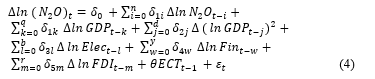
where represents the nitrous oxide emissions in Bahrain. The above function shows that the explanatory variables for nitrogen oxide emissions are the economic growth (GDP), square of economic growth ( ), electricity consumption (Elec), financial developments (Fin) and foreign direct investments (FDI).

Looking at the main objective of this study, it is suggested to derive a natural log form equation from the above linear equation, so it allows for testing the hypothesis of the EKC. Having natural log model ensure the production of reliable and effective results. Furthermore, in [41], the authors have reported that a natural log model will help in satisfying the stationary condition of the variance-covariance matrix. Accordingly, re-writing the model above can be represented by the following equation:

where is the error term associated with the estimation while is the intercept. The coefficients  represent, respectively, the impacts of GDP per capita and its quadratic term, electricity consumption per capita, financial developments, and the percentage of foreign direct investments. Based on the theory of EKC, it is likely that  has positive sign while  has a negative sign.

Having a glance at (2) shown above, it is revealed that none of GDP term or its square term can be excluded. The aim of adding both terms in the same equation is to investigate the authenticity of the EKC, which can be verified only if the relationship among environmental emissions and economic growth is expressed by an inverted U-shape curve. In another words, if the relationship among the environmental emissions and economic growth is an inverted U-shape, EKC hypothesis cannot be rejected. Therefore, the environmental emissions will tend to increase as much as there is an increase in output per capita, until it reaches to a specific level (peak). Accordingly, the quality of the environment will be better.

In a study conducted by [6], it is reported that if there is no significant change in technology in an economy, it is expected that an inverted U-shape curve represents the linkage between GDP per capita and the emissions of the environment. Precisely, an expansion of an economy causes negative impacts on environment at early stages. However, as much as it grows, structural change is experienced by the economy due to many factors including information intensive industries and services, advances in technology, increase in environmental consciousness and implementation of environmental protocols, which may have positive influence on reducing environmental emissions.

3.3. ARDL Approach

The purpose of this study is to investigate the hypothesis of having an environmental Kuznets curve, that be represents a curve of an inverted U-shape to express the linkage between the emissions of environment and the growth of an economy. Accordingly, long- and short-term dynamics of the model can be investigated using a cointegration approach named Autoregressive Distributed Lag Model (ARDL). Among others, the authors of [42], [43], [44], and [45] have used ARDL, which starts as a general model and then moves into more specific one to capture the characteristics of the data included in the regression using a sufficient number of lags. As literature has discussed many advantages for using ARDL in cointegration models, it is worth to shed the light on some key advantages that have affected the selection of the model for this study. First, in [42], the author has reported that the ARDL approach is suitable for variables with different integration orders that could be either fractional or at I (0) or I (1). In addition, the equilibrium features of both short- and long-term dynamics are captured by the error correction model (ECM) which is obtained from a transformation that is done linearly for the ARDL model.

Considering the size of the sample, the authors of [44] have claimed that when the investigation is done on a small sample, then the approach of ARDL is more appropriate in comparison to that of [46] cointegration. They have also admitted that ARDL has minimal residual correlation and thus considered as a superior approach against serial correlation problems attributed to endogeneity issue. Lastly, being able to proceed with the estimation even if the explanatory variables are endogenous is another key advantage of ARDL model [42], [45].

3.4. Unit Root Testing

As time series data exhibit trending behavior and thus the null hypothesis of non-stationary cannot be rejected, unit root testing is applied using three different approaches called Augmented Dickey & Fuller (ADF) [47], Phillips and Perron (PP) [48] and KPSS [49] to test the order of integration of each variable. In fact, both ADF and PP tests suggest that the null hypothesis is non-stationary where KPSS claims a stationary null hypothesis. Since the original Dickey & Fuller test [47] cannot accommodate complex models, the ADF approach is a customized version of the test that can satisfy the need of having an appropriate stationary test for complex models. The ADF for models with unknown orders can be represented as shown below:

where is the variable in period t; ∆ is the – ;  the disturbance term represented by  is i.i.d and has zero mean where the variance is 1; t the linear time trend and p is the lag order. It is worth to note that the ADF test has been developed to examine univariate time series for the presence of unit root. In another word, any time series with presence of unit root should be treated to ensure that the variable is stationary (if it is required for modelling).

Since  and  are the coefficients of the time trend term (t) and the variable  in previous period (t-1), it is important to investigate the order of integration of the variable . This is done by examining whether or not  = 0 in (3). Accordingly, if  is not significantly less than zero, the null hypothesis of a unit root cannot be rejected. Otherwise, both level and first differenced variables are tested against unit root. Since in [49], the KPSS stationary test was introduced which assumes that stationary is the null hypothesis, this study has also applied this test to make sure that the results are superior.

3.5. Bound Testing Approach

The next step after getting the order of integration for each variable under concern, the ARDL bound testing [45] is implemented to investigate the existence of long run association between the variables. The ARDL bound testing depends on assessing the joint significance of the lagged variables coefficients using F-Wald test, which has a null hypothesis of H0:  =  =  =  =  = 0, whereas the alternative is that at least one coefficient ( ) is not equal to zero.  There are upper and lower critical values that should be compared with the results obtained from the F-statistics, where all are tabulated by [45]. There will be a proof of cointegration with a presence of long run association between the variables if the estimated F-statistic is more than the upper limit. If the computed F-statistic falls between the two critical limits, no conclusion can be provided by the test. However, the null hypothesis cannot be rejected if the values of F-statistic is less than the lower limit. In addition, this applies that there is no existence of cointegration among the tested variables.

If the estimated F-statistic shows the presence of long run relationship between the variables, the next stage of the ARDL specification is estimating the long run coefficients in (2) [50].  The long run impact on the N₂O emissions is measured by the estimated values of . The Akaike Information Criteria (AIC) [51] is utilized to decide on the optimal lag length for each variable.

The residuals obtained from estimating (2) are used to approximate the error correction term (ECT), which shows the speed that the variables restore to their equilibrium levels in the long run from the short run. Therefore, the value of the coefficient of ECT should be negative and less than or equal to one besides being highly significant. Hence, the specifications of the error correction term of the ARDL approach can be estimated as follows:

where   represents the growth or changes in N₂O emissions , GDP per capita (  and its quadratic term, electricity consumption per capita ( , financial developments ( , and the percentage of foreign direct investments ( . The term of reflects the speed of adjustment when a deviation take place. The value of the is negative.

4. Empirical Results and Discussion

Before estimating any time series model, it is essential to examine the integration order of the variables and identify their order of integration. This study employs ADF test, KPSS test and PP test. The results of the three tests are reported in Table 2 which reveals that all the variables except the FDI are having unit root at level however a first difference convert them to stationary variables. Hence, the integration order is 1; i.e. I (1).

Table 2: Unit root results

Variable	ADF		KPSS		PPerron
	Constant	Constant and Trend	Constant	Constant and Trend	Constant	Constant and Trend
lnN2O	-2.33	-3.93**	0.48**	0.14*	-3.01**	-4.10*
lnGDPpc	-1.07	-2.33	0.31	0.11	-1.29	-2.55
lnElec	-3.23**	-2.55	0.37	0.15**	-3.65**	-2.57
Fin	-0.11	-3.04	0.46**	0.15**	0.22	-2.99
FDI	-5.51***	-5.48***	0.29	0.15**	-5.61***	-5.55***
ΔlnN2O	-7.49***	-8.35***	0.32	0.11	-7.37***	-8.45***
ΔlnGDpc	-4.74***	-4.63***	0.14	0.11	-4.76***	-4.62***
ΔlnElec	-5.24***	-5.69***	0.35	0.15**	-5.23***	-5.73***
ΔFin	-5.83***	-5.74***	0.29	0.13	-6.02***	-5.92***
ΔFDI	-8.05***	-7.94***	0.31	0.17**	-11.2***	-11.1***
Notes: ADF is the Augmented Dickey Fuller Unit root test, KPSS is the Kwiatkowski, Phillips, Schmidt & Shin stationarity test. PP is Phillips & Perron unit root test. lnN2O is the natural logarithm of nitrous oxide emissions, lnGDPpc is the natural logarithm of GDP per capita, lnElec is the natural logarithm of electric power consumption, Fin is the Domestic credit provided by Financial Sector (% of GDP) and FDI is Foreign direct investment, net inflows (% of GDP). Δ is the first difference. *, ** and *** show 10%, 5% and 1% level of significance, respectively.

The findings obtained from stationary tests serve as the basics to implement the following steps of estimation. In order to explore the presence of long run relationship among the N₂O emissions and its determinants, the bound testing method of ARDL that aims for exploring cointegration is employed in (4) and the results are shown in Table 3. AIC is utilized in selecting the optimal lag structure for all the variables and the results are as (1,0,0,0,2,0) for the function . The estimated F statistic is 10.052 which is greater than the value of the upper critical limit developed by [52]. Therefore, it is possible that the null hypothesis of no cointegration is rejected.

Table 3: Results of ARDL bound testing to cointegration

Model	Optimal lag structure	F – value	t – statistics
	(1,0,0,0,2,0)	10.052	-6.77***

Table 4: Estimated Coefficients from ARDL (1,0,0,0,2,0) for Model

Long run estimates:   as dependent variable	Variable	Coefficients		t-statistics
			4.5	2.18**
			-2.3	-2.20**
			0.66	2.74**
			-0.20	-4.64***
			-0.40	-1.33*
Short run estimates:  as dependent variable			2.30	2.42**
			-4.6	-2.44**
			0.72	2.36**
			-0.10	-1.29
			0.40	3.60**
			-0.20	-0.33
			-0.76	-6.77***
	Constant		14.43	1.54
	trend		-0.44	-6.97***

Table 5: Diagnostic Tests

Test	Coefficient
	0.76
Adjusted	0.66
F- statistics	10.052(0.023)
Jarque-Bera normality test	1.062(0.334)
Heteroscedasticity Test: ARCH	2.83(0.984)
Breusch-Godfrey Serial Correlation LM Test	0.718(0.315)
Ramsey RESET test	0.723(0.413)

Table 4 presents the findings of ARDL estimation. The upper part of Table 4 illustrates the coefficients of the long run relationship. All the estimated coefficients appear to have significant impacts on N₂O emission at 1% or 5% level of significance except the coefficient of FDI, which is only significant at 10% level. Specifically, the GDP per capita elasticity is statistically significant and has a positive sign in both long and short run relationships. Moreover, the coefficient of the squared GDP per capita turned out to be negative and significant in both timeframes. The negative coefficient on the squared value of GDP per capita confirms the presence of the Environmental Kuznets Curve (EKC), which indicates the relationship between Bahrain economic growth and the level of N₂O emissions follows the inverted U-shape curve in the long run.

The findings of Table 4 demonstrate the coefficients of the other variables under concern. A 1% increase in electricity consumption causes 0.66% surge in N₂O diffusion. However, foreign direct investments and financial development variables are negatively related to the N₂O emissions as they cause a decrease in N₂O emissions of 0.4% and 0.2%, respectively. This is a good sign for policy makers to consider the improvement in the financial sector and draw the attention of foreign direct investments, which may help boosting air quality in Bahrain. Furthermore, the electricity consumption variable occurs to have a negative significant impact on N₂O emissions level.

The lower part of Table 4 reveals the findings of the short run estimations of the dynamic effects on N₂O diffusions by its determinants. The Δ sign implies that the variables are in their first differences.  Briefly, for the error correction term (ECT_t-1), the coefficient is not only negative (as expected) but also significant at 5% level. This reinforces the hypothesis of cointegration and gives a measure for the how fast is the adjustment to equilibrium in the short run, which is around 76% in a year.

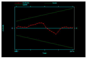Figure 1: Plot of Cumulative Sum of Recursive Residuals

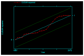Figure 2: Plot of Cumulative Squared Sum of Recursive Residuals

To reassure the stability of the obtained findings, Table 5 reports the results obtained from some diagnostic tests that are applied for ARDL estimations. The findings prove that there is no serial correlation in the residuals, and the distribution is normal. Moreover, the variance of the errors is constant (homoscedastic). Furthermore, the cumulative sum of recursive residuals (CUSUM) and the cumulative squared sum of recursive residuals (CUSUMSQ) established by [53] are plotted in Figures 1 and 2 to examine the model’s parameters stability. Figures 1 and 2 illustrate the stability of the estimated model as both plots occur within the limits of the 5% confidence interval. It is important to check the stability of the model for it to be strong enough for forecasting issues and accordingly applicable for policies implementations.

5. Conclusion and Recommendations

This paper examines the validity of the EKC hypothesis in Bahrain over the period 1980 – 2012 with the implication of nitrous oxide (N₂O) emissions as an environmental pollutant. The estimated equation is augmented with electric power consumption, foreign direct investment and financial development indicator. ARDL approach is employed to examine the short and long run impact of the variables under interest on N₂O emissions. The obtained results from the ARDL estimation indicate the validity of the EKC hypothesis. Moreover, electric power consumption has a positive impact on N₂O emissions in the short and long run. However, foreign direct investments and financial development have negative impact on the emissions of N₂O.

In order to decrease the impact of electric power consumption on N₂O emissions, Bahrain should continue its efforts in decreasing the environmental emissions such as assisting households to install solar cells on the top of their houses and use solar energy in generating their own need for electricity, which may help in reducing the electricity production using fossil fuel combustion.

Although the authors of [36] and [37] argue that foreign investors and international corporations prefer investing in countries that have loose environmental policies and standards as most of these investments sponsor forms of production that are environmentally inefficient [38], this paper found that FDI reduces N₂O emissions. Our results are in line with that of [54] who found that FDI can be good for the environment. They explain this relationship by referring to the possibility of transferring the foreign firms’ green technologies to their domestic counterparts which may have low environmental-friendly technologies.  As the FDI helps decreasing N₂O emissions, Bahrain should increase its focus on the quality of FDI to be technology oriented FDI. Moreover, the financial development indicator reduces the N₂O emissions. Therefore, Bahrain should enhance its financial sector by developing bond and securities markets. This will improve the financial services and provide more funds to be invested in research and development on new and advanced techniques to generate clean energy.

Acknowledgment

Authors would like to thank the referees for their useful comments and support.

[3] GDP at purchaser’s prices is the sum of gross value added by all resident producers in the economy plus any product taxes and minus any subsidies not included in the value of the products. It is calculated without making deductions for depreciation of fabricated assets or for depletion and degradation of natural resources. Data are in constant 2010 U.S. dollars.

[4] The most available data for N₂O were till the year 2012.

1. R.J. Hill, E. Magnani, “An exploration of the conceptual and empirical basis of the environmental Kuznets curve,” Australian Economic Papers, 41(2), 239–254, 2002. https://doi.org/10.1111/1467-8454.00162
2. M.D. Miah, M.F.H. Masum, M. Koike, “Global observation of EKC hypothesis for CO2, SOx and NOx emission: A policy understanding for climate change mitigation in Bangladesh,” Energy Policy, 38(8), 4643–4651, 2010. https://doi.org/10.1016/j.enpol.2010.04.022
3. M.A. Zambrano?Monserrate, M.A. Fernandez, “An environmental Kuznets curve for N2O emissions in Germany: an ARDL approach,” in Natural resources forum, Wiley Online Library: 119–127, 2017. https://doi.org/10.1111/1477-8947.12122
4. A.M. Rasli, M.I. Qureshi, A. Isah-Chikaji, K. Zaman, M. Ahmad, “New toxics, race to the bottom and revised environmental Kuznets curve: The case of local and global pollutants,” Renewable and Sustainable Energy Reviews, 81, 3120–3130, 2018. https://doi.org/10.1016/j.rser.2017.08.092
5. G.M. Grossman, A.B. Krueger, Environmental impacts of a North American free trade agreement, National Bureau of economic research Cambridge, Mass., USA, 1991.
6. T. Panayotou, Empirical tests and policy analysis of environmental degradation at different stages of economic development, International Labour Organization, 1993.
7. S. Farhani, M. Shahbaz, R. Sbia, A. Chaibi, “What does MENA region initially need: grow output or mitigate CO2 emissions?,” Economic Modelling, 38, 270–281, 2014. https://doi.org/10.1016/j.econmod.2014.01.001
8. L.-S. Lau, C.-K. Choong, Y.-K. Eng, “Investigation of the environmental Kuznets curve for carbon emissions in Malaysia: do foreign direct investment and trade matter?,” Energy Policy, 68, 490–497, 2014. https://doi.org/10.1016/j.enpol.2014.01.002
9. S. Oshin, A. Ogundipe, “An empirical examination of environmental Kuznets curve (EKC) in West Africa,” Euro-Asia Journal of Economics and Finance, 3(1), 2014. https://ssrn.com/abstract=2512136
10. N. Apergis, “Environmental Kuznets curves: New evidence on both panel and country-level CO2 emissions,” Energy Economics, 54, 263–271, 2016. https://doi.org/10.1016/j.eneco.2015.12.007
11. S. Park, Y. Lee, “Regional model of EKC for air pollution: Evidence from the Republic of Korea,” Energy Policy, 39(10), 5840–5849, 2011. https://doi.org/10.1016/j.enpol.2011.06.028
12. O.A. Onafowora, O. Owoye, “Bounds testing approach to analysis of the environment Kuznets curve hypothesis,” Energy Economics, 44, 47–62, 2014. https://doi.org/10.1016/j.eneco.2014.03.025
13. S. Özokcu, Ö. Özdemir, “Economic growth, energy, and environmental Kuznets curve,” Renewable and Sustainable Energy Reviews, 72, 639–647, 2017. https://doi.org/10.1016/j.rser.2017.01.059
14. E.L. Effiong, A.O. Iriabije, “Let the data speak: semiparametric evidence on the environmental Kuznets curve in Africa,” Quality & Quantity, 52(2), 771–782, 2018. https://doi.org/10.1007/s11135-017-0487-6
15. M. Fodha, O. Zaghdoud, “Economic growth and pollutant emissions in Tunisia: an empirical analysis of the environmental Kuznets curve,” Energy Policy, 38(2), 1150–1156, 2010. https://doi.org/10.1016/j.enpol.2009.11.002
16. C.-H. Cho, Y.-P. Chu, H.-Y. Yang, “An environment Kuznets curve for GHG emissions: a panel cointegration analysis,” Energy Sources, Part B: Economics, Planning, and Policy, 9(2), 120–129, 2014. https://doi.org/10.1080/15567241003773192
17. L. Charfeddine, Z. Mrabet, “The impact of economic development and social-political factors on ecological footprint: A panel data analysis for 15 MENA countries,” Renewable and Sustainable Energy Reviews, 76, 138–154, 2017. https://doi.org/10.1016/j.rser.2017.03.031
18. Y. Chiu, “Deforestation and the environmental Kuznets curve in developing countries: A panel smooth transition regression approach,” Canadian Journal of Agricultural Economics/Revue Canadienne d’agroeconomie, 60(2), 177–194, 2012. https://doi.org/10.1111/j.1744-7976.2012.01251.x
19. K. Ahmed, M. Shahbaz, A. Qasim, W. Long, “The linkages between deforestation, energy and growth for environmental degradation in Pakistan,” Ecological Indicators, 49, 95–103, 2015.
20. M. Mazzanti, A. Montini, R. Zoboli, “Municipal waste generation and the EKC hypothesis new evidence exploiting province-based panel data,” Applied Economics Letters, 16(7), 719–725, 2009. https://doi.org/10.1080/13504850701221824
21. P.K. Narayan, S. Narayan, “Carbon dioxide emissions and economic growth: Panel data evidence from developing countries,” Energy Policy, 38(1), 661–666, 2010. https://doi.org/10.1016/j.enpol.2009.09.005
22. Z. Zoundi, “CO2 emissions, renewable energy and the Environmental Kuznets Curve, a panel cointegration approach,” Renewable and Sustainable Energy Reviews, 72, 1067–1075, 2017. https://doi.org/10.1016/j.rser.2016.10.018
23. S. Sinha Babu, S.K. Datta, “The relevance of environmental Kuznets curve (EKC) in a framework of broad-based environmental degradation and modified measure of growth–a pooled data analysis,” International Journal of Sustainable Development & World Ecology, 20(4), 309–316, 2013. https://doi.org/10.1080/13504509.2013.795505
24. F. Abbasi, K. Riaz, “CO2 emissions and financial development in an emerging economy: an augmented VAR approach,” Energy Policy, 90, 102–114, 2016. https://doi.org/10.1016/j.enpol.2015.12.017
25. S. khoshnevis Yazdi, B. Shakouri, “The renewable energy, CO2 emissions, and economic growth: VAR model,” Energy Sources, Part B: Economics, Planning, and Policy, 13(1), 53–59, 2018. https://doi.org/10.1080/15567249.2017.1403499
26. U. Al-Mulali, S.A. Solarin, I. Ozturk, “Investigating the presence of the environmental Kuznets curve (EKC) hypothesis in Kenya: an autoregressive distributed lag (ARDL) approach,” Natural Hazards, 80(3), 1729–1747, 2016. https://doi.org/10.1007/s11069-015-2050-x
27. E. Dogan, B. Turkekul, “CO 2 emissions, real output, energy consumption, trade, urbanization and financial development: testing the EKC hypothesis for the USA,” Environmental Science and Pollution Research, 23(2), 1203–1213, 2016. https://doi.org/10.1007/s11356-015-5323-8
28. W. Ali, A. Abdullah, M. Azam, “Re-visiting the environmental Kuznets curve hypothesis for Malaysia: fresh evidence from ARDL bounds testing approach,” Renewable and Sustainable Energy Reviews, 77, 990–1000, 2017. https://doi.org/10.1016/j.rser.2016.11.236
29. U.K. Pata, “Renewable energy consumption, urbanization, financial development, income and CO2 emissions in Turkey: testing EKC hypothesis with structural breaks,” Journal of Cleaner Production, 187, 770–779, 2018. https://doi.org/10.1016/j.jclepro.2018.03.236
30. B. Raggad, “Carbon dioxide emissions, economic growth, energy use, and urbanization in Saudi Arabia: evidence from the ARDL approach and impulse saturation break tests,” Environmental Science and Pollution Research, 25(15), 14882–14898, 2018. https://doi.org/10.1007/s11356-018-1698-7
31. A.S. Alshehry, M. Belloumi, “Study of the environmental Kuznets curve for transport carbon dioxide emissions in Saudi Arabia,” Renewable and Sustainable Energy Reviews, 75, 1339–1347, 2017. https://doi.org/10.1016/j.rser.2016.11.122
32. H. Mahmood, T.T.Y. Alkhateeb, “Trade and environment nexus in Saudi Arabia: An environmental Kuznets curve hypothesis,” International Journal of Energy Economics and Policy, 7(5), 291–295, 2017. https://EconPapers.repec.org/RePEc:eco:journ2:2018-03-5
33. M. Shahbaz, R. Sbia, H. Hamdi, I. Ozturk, “Economic growth, electricity consumption, urbanization and environmental degradation relationship in United Arab Emirates,” Ecological Indicators, 45, 622–631, 2014. https://doi.org/10.1016/j.ecolind.2014.05.022
34. L. Charfeddine, K. Ben Khediri, “Financial development and environmental quality in UAE: Cointegration with structural breaks,” Renewable and Sustainable Energy Reviews, 55, 1322–1335, 2016. https://doi.org/10.1016/j.rser.2015.07.059
35. Z. Mrabet, M. Alsamara, “Testing the Kuznets Curve hypothesis for Qatar: A comparison between carbon dioxide and ecological footprint,” Renewable and Sustainable Energy Reviews, 70, 1366–1375, 2017. https://doi.org/10.1016/j.rser.2016.12.039
36. N.D. Woods, “Interstate competition and environmental regulation: a test of the race?to?the?bottom thesis,” Social Science Quarterly, 87(1), 174–189, 2006. https://doi.org/10.1111/j.0038-4941.2006.00375.x
37. C. Dick, A.K. Jorgenson, “Sectoral foreign investment and nitrous oxide emissions: A quantitative investigation,” Society & Natural Resources, 23(1), 71–82, 2009. https://doi.org/10.1080/08941920802392690
38. P. Grimes, J. Kentor, “Exporting the greenhouse: foreign capital penetration and CO? Emissions 1980 1996,” Journal of World-Systems Research, 261–275, 2003.
39. U. Soytas, R. Sari, B.T. Ewing, “Energy consumption, income, and carbon emissions in the United States,” Ecological Economics, 62(3–4), 482–489, 2007. https://doi.org/10.1016/j.ecolecon.2006.07.009
40. M. Shahbaz, M.M. Rahman, “Foreign capital inflows-growth nexus and role of domestic financial sector: an ARDL co-integration approach for Pakistan,” Journal of Economic Research, 15(3), 207–231, 2010.
41. T. Chang, W. Fang, L.-F. Wen, “Energy consumption, employment, output, and temporal causality: evidence from Taiwan based on cointegration and error-correction modelling techniques,” Applied Economics, 33(8), 1045–1056, 2001. 10.1080/00036840122484
42. M.H. Pesaran, “The role of economic theory in modelling the long run,” The Economic Journal, 107(440), 178–191, 1997. https://www.jstor.org/stable/2235280
43. M.H. Pesaran, R.P. Smith, “Structural analysis of cointegrating VARs,” Journal of Economic Surveys, 12(5), 471–505, 1998. https://doi.org/10.1111/1467-6419.00065
44. H.H. Pesaran, Y. Shin, “Generalized impulse response analysis in linear multivariate models,” Economics Letters, 58(1), 17–29, 1998. https://doi.org/10.1016/S0165-1765(97)00214-0
45. M.H. Pesaran, Y. Shin, R.J. Smith, “Bounds testing approaches to the analysis of level relationships,” Journal of Applied Econometrics, 16(3), 289–326, 2001. https://doi.org/10.1002/jae.616
46. S. Johansen, K. Juselius, “Maximum likelihood estimation and inference on cointegration—with appucations to the demand for money,” Oxford Bulletin of Economics and Statistics, 52(2), 169–210, 1990. https://doi.org/10.1111/j.1468-0084.1990.mp52002003.x
47. D.A. Dickey, W.A. Fuller, “Distribution of the estimators for autoregressive time series with a unit root,” Journal of the American Statistical Association, 74(366a), 427–431, 1979. https://doi.org/10.1080/01621459.1979.10482531
48. P.C.B. Phillips, P. Perron, “Testing for a unit root in time series regression,” Biometrika, 75(2), 335–346, 1988. https://doi.org/10.1093/biomet/75.2.335
49. D. Kwiatkowski, P.C.B. Phillips, P. Schmidt, Y. Shin, “Testing the null hypothesis of stationarity against the alternative of a unit root: How sure are we that economic time series have a unit root?,” Journal of Econometrics, 54(1–3), 159–178, 1992. https://doi.org/10.1016/0304-4076(92)90104-Y
50. M. Bouznit, M. del P. Pablo-Romero, “CO2 emission and economic growth in Algeria,” Energy Policy, 96, 93–104, 2016. https://doi.org/10.1016/j.enpol.2016.05.036
51. Y. Sakamoto, M. Ishiguro, G. Kitagawa, “Akaike information criterion statistics,” Dordrecht, The Netherlands: D. Reidel, 81(10.5555), 26853, 1986. https://doi.org/10.1080/01621459.1988.10478680
52. P.K. Narayan, “The saving and investment nexus for China: evidence from cointegration tests,” Applied Economics, 37(17), 1979–1990, 2005. https://doi.org/10.1080/00036840500278103
53. R.L. Brown, J. Durbin, J.M. Evans, “Techniques for testing the constancy of regression relationships over time,” Journal of the Royal Statistical Society: Series B (Methodological), 37(2), 149–163, 1975. https://doi.org/10.1111/j.2517-6161.1975.tb01532.x
54. B.A. Demena, S.K. Afesorgbor, “The effect of FDI on environmental emissions: Evidence from a meta-analysis,” Energy Policy, 138, 111192, 2020. https://doi.org/10.1016/j.enpol.2019.111192

(Click Here)