1. Introduction

1.1. Literature Review

Classical gradient-based optimization algorithms [1], [2] require at least first-order gradient information to minimize/ maximize the objective function. If the objective function can be written as a mathematical function, then the gradient can be derived analytically. For a complex physics simulator, such as finite element method (FEM), computational fluid dynamics (CFD), and multibody dynamics (MBD), gradients are not readily available to perform design optimization. To overcome this problem, a data-driven approach, such as response surface methodology or surrogate modelling [3], is applied to model the simulator’s behavior, and the gradients are obtained rapidly. The response surface methodology and surrogate modeling approximate the relationship between design variables (inputs) and the objective values (outputs). Once the approximated model is constructed, gradient information for optimization are much cheaper to evaluate. However, this approach may require many precomputed data points to construct an accurate model depending on the dimensionality of the actual system. Therefore, generating many data points arises as one of the bottlenecks of this method in practice due to the high computational cost of physics simulations.

In addition, the data-driven approach may not generalize the behavior of the physics simulation accurately. This would cause the approximated model to produce invalid solutions throughout the design space except at the precomputed data points. This will be detrimental in optimization, where the best solution must be found among all true solutions.

A possible reason data-driven approach fails is its reliance on the function approximator to learn the underlying physical relationships using a finite amount of data points. In theory, a function approximator can predict the relationship between any input and output according to the universal approximation theorem [4], [5]. However, this usually requires enough capacity and complexity of the function and sufficient data points to train the function. These data points are expensive to obtain and a significant amount of effort must be placed towards computing the objective values of each data point through a physics simulator. In the end, only the design variables and corresponding objective values are paired for further analysis (surrogate modeling and optimization). All the information during the physics simulation is discarded and wasted. Many ideas have been proposed to solve topology optimization using data-driven approach. In [6], [7] the showed the GAN’s capability of generating new structure topologies. In [8], the authors proposed a TopologyGAN to generate a new structure design given arbitrary boundary and loading conditions. In [9], the authors designed a GAN framework to generate a new airfoil shape. All these approaches are data-driven methods where large dataset must be prepared to train the neural network for surrogate modeling.

To use the computational effort during physical simulations, we turn to a newly emerged idea called differential programming [10], [11] which applies automatic differentiation to calculate the gradient of any mathematical/ non-mathematical operations of a computer program. Because of this, we can make the physics model be fully differentiable and integrate it with a deep neural network and use backpropagation for training. In [12], the authors discussed the application of automatic differentiation on density-based topology optimization using existing software packages. In [13], [14] the authors demonstrated the ability to use automatic differentiation to calculate gradients for fluid and heat transfer optimization. Furthermore, in [15] the authors modeled the solution of a partial differential equation (PDE) as an unknown neural network. Plugging the neural network into the PDE forces the neural network to follow the physics governed by the PDE. A small amount of data is required to train the neural network to learn the real solution of the PDE. In [16], [17] the authors demonstrated the application of a physics-informed neural network on high-speed flow and large eddy simulation. In [18], the authors designed an NSFnet based on a physics-informed neural network to solve incompressible fluid problems governed by Navier-Stokes equations. In this work, we will design optimal structural topology by integrating the neural network and the physics model(FEM) into one training process. The FE model is made fully differentiable through automatic differentiation to provide critical gradient information for training the neural network.

1.2. Review of Solid Isotropic Material with Penalization Method (SIMP)

The SIMP method proposed by Bendsoe [19] established a procedure (Figure 1) for density-based topology optimization.

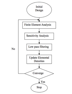Figure 1: SIMP Method Optimization Process

The algorithm begins with an initial design by filling in a value  in each quadrilateral element of a predefined structured mesh in a fixed domain. The value represents the material density of the element where  means a void and 1 means filled. A value between  and  is partially filled, which does not exist in reality. It makes optimization easy but results in a blurry image of the design. Therefore, the author [19] proposed to add a penalization factor to push the element density towards either void or completely filled.

The objective of the SIMP method is to minimize the compliance, , of the design domain under fixed loadings and boundary conditions. The compliance defined in (1), also described as total strain energy, is a measure of the overall displacement of a structure.

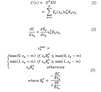Inside the optimization loop, the density of each element  has to be updated to lower the compliance. For a gradient-based method, the gradient  is calculated as (2) by taking a derivative of (1). Then a heuristic update rule, (3), is crafted to ensure the optimality condition is satisfied for the design. In other popular density-based topology optimization techniques, such as level-set [20], [21] or bidirectional evolutionary optimization [22] an analytical formula of gradient, element density derivative, or shape derivative must be provided manually. In the proposed framework in Section 2, there is no need to provide such gradient information analytically as the gradients are calculated by reverse mode automatic differentiation.

1.3. Motivation

In this work, the goal is to integrate a physics-based model (e.g., finite element model) with a neural network for generating feasible topology designs so that the gradient information obtained from the finite element model can be used to minimize the loss function during the training process to achieve optimal topology designs. The critical gradient information and update rules are determined using automatic differentiation and ADAM optimizer, eliminating hand-coded equations, such as (5) and (6). Furthermore, the critical gradient information directly obtained in the finite element model would contain essential features which may not exist or are significantly diluted in the training data sets.

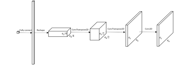Figure 2: Generator Neural Network Architecture

In addition, the proposed approach does not require a significant amount of time for preparing the training data set.

In Section 2, we have constructed a new topology optimization procedure by integrating a deep learning neural network with a wildly used classical SIMP topology optimization method to achieve efficiency and flexibility. This integrated physics-informed deep learning optimization process is presented in Section 2 and has been implemented in Julia programming language, which can be automatically differentiated in reverse mode for gradient calculations. The proposed integrated deep learning and topology optimization approach has been demonstrated on several famous 2-D topology optimization test cases, which were found to be a good agreement with the SIMP method. Further validation of the idea and approach via complex structural systems and boundary and/or loading conditions will be conducted in our future work.

2. Proposed Physic-Informed Deep Learning Process

2.1. Mathematical Formulation

In this work, we will perform the topology optimization with integrated physics-informed neural network. The neural network is physics-informed because its parameters are updated using gradient information directly from the finite element model.

A flow chart of the proposed physics-informed deep learning design optimization procedure is outlined in Figure 2. The equivalent mathematical formulation can be stated as:

                               subject to:

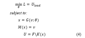The  is the displacement at the applied load point and it is the loss function, L, to be minimized. The input to the generator is the target mass fraction, . The generator, , is a deep neural network with parameter  and it outputs a topology, x, based on the target mass fraction. The  returns the mass fraction of the topology produced by generated and compare it to the target mass fraction. The  and F are the stiffness matrix of the topology and load vector, respectively. They are processed in the FEM component in Figure 2, and a resultant displacement U is returned.

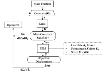Figure 3: Proposed Physics-Informed Deep Learning Topology Optimization Approach

Instead of providing a hand-coded gradient equation, (1.2), and update rule, (1.3), the gradient of every operation throughout the calculation is determined by using reverse differentiation (ReverseDiff). The gradient is a vector of , where  is a scalar value of the objective function.  In the examples shown in Section 4, the compliance/displacement is the objective function, while a given total mass is equality constrain that must be satisfied. Instead of providing an update rule, the generator, G(.), proposes a new design (x) for every iteration. The parameters of the network are adjusted simultaneously to generate better design while satisfying the mass constraint. Therefore, in the proposed algorithm, the gradients that guide the design approaching optimal are not , but   instead. For a 1-D design case where the design variables have no spatial dependencies, the neural network is a multilayer perceptron. While for 2D cases, the neural network architecture is composed of layers of the convolutional operator, which is good at learning patterns of 2-D images. Thus, the objective of this topology optimization becomes learning a set of parameters, θ, such that the generator can generate a 2D structure, x, such that it minimizes the displacement at the point of load while satisfying the mass constraint.

The optimizer component in Figure 2 is the algorithm to update the variables given the gradient information. In this work, ADAM (ADAptive Moments) [23] is used to handle the learning rate and update the parameter θ of the generator in each iteration.

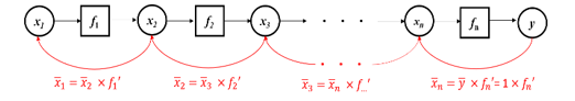Figure 4: A Computation Graph of a Single-Input-Single-Output Function

2.2. Generator Architecture

The network architecture of the generator in is illustrated in Figure 3. Adapting the idea of the generator from Generative Adversarial Network (GAN) [24], which can generate high-quality images after training, the generator starts with a seed value (fixed or random) which followed by a fully connected layer. Then the fully connected layers are reshaped to a feature layer composed of a 3D array. The first two dimension relate to the feature layer’s width and height, and the third dimension refers to channels. Then the following components are to expand the width and height of the feature layer but shrink the number of channels down to 1. In the end, the output will be a 2D (3^rd   dimension is 1) image with correct size  based on the learnable parameter θ. In Figure 3, the output size of the ConvTranspose2D layer doubles every time. The second last layer has an activation function, , making sure the output values are bounded. The last convolutional layer does not change the size of the input, and its parameters are predetermined and kept fixed. The purpose of the last layer is to average the density value around the neighborhood of each element to eliminate the checkerboard pattern. This is similar to the filtering technique used in the SIMP method [25], [26].

The generator architecture can vary by adding more layers or new components. Instead of starting with a size of , one can make this even smaller and add more channels at the beginning. Hyper-parameters such as the kernel sizes and activation functions can be applied to any layers of the generator. However, in this paper, the architecture design is kept simple without experimenting too much with the hyper-parameters.

3. Automatic Differentiation

The idea of automatic differentiation uses derivative rules of general operations to calculate the derivatives of outputs to inputs of a composite function  , where  and  are the dimensions of inputs and outputs, respectively. In general, the resulting derivatives form an  Jacobian matrix. When  , the derivatives form a gradient vector with length . The automatic differentiation can be done in two ways: forward mode [27] or reverse mode [11]. In the following, ForwardDiff and ReverseDiff will be used for short. Usually, the entire composite function F has no simple derivative rule associated with it. However, since it can be decomposed into other functions or mathematical operations where the derivatives are well defined, the chain rule can be applied to propagate the derivative information either forward (ForwardDiff) or backward (ReverseDiff) through the computation graph of a composite function . The ForwardDiff has linear complexity with respect to the input dimension, and therefore, it is efficient for a function when . Further detail of the forward differentiation can be found in reference [27]. Conversely, the ReverseDiff is ideal for a function when , and applied in this paper to calculate derivatives. ReverseDiff can be taken advantage of in this situation as the dimension of the inputs (densities of each element) is very large, but the output dimension is just one scalar value, such as overall compliance or displacement.

3.1. Reverse Mode Differentiation (ReverseDiff)

The name, ReverseDiff, comes from a registered Julia package called ReverseDiff.jl and additionally has a library of well-defined rules for reverse mode automatic differentiation. The idea of ReverseDiff is related to the adjoint method [11], [20], [28], [29] and applied in many optimization problems where the information from the forward calculation of the objective function is reused to calculate the gradients efficiently. In structure optimization, the adjoint method solves an adjoint equation  [30], [31]. Since  is known when solving   during the forward pass, then the adjoint equation can be solved with a small computational cost without factorizing or calculating the inverse of matrix again. The ReverseDiff is also closely related to backpropagation [32] for training a neural network in machine learning. The power of ReverseDiff is that it takes the automatic differentiation into a higher level, where any operation (mathematical or not mathematical) can be assigned with a derivative rule (called pullback function). Then with the chain rule, we can combine the derivatives of every single operation and compute the gradient from end to end of any black-box function, i.e., physics simulation engine or computer program. To formulate the process for ReverseDiff, a composite function :  is considered, where any intermediate step can be written as  A computation graph of the composite function is shown in Figure 4. For simplicity, it is assumed that any intermediate function inside the composite function is a single input and a single output.

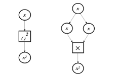Figure 5: Computation Graphs of x² (left) and x*x (right)

The black arrows are the forward pass for function evaluations, and the red arrows are reverse differentiation with chain rule been applied. The idea can be generalized to multiple inputs and outputs as well. To ReverseDiff of the function from end to end in Figure 4, we will define and expand derivative using chain rule as:

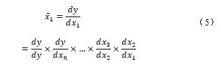On the right side of the (3.1), y is called seed, and its value equals 1. Starting from the last node, y, it essentially calculates  as going backward through the computation graph. It can be shown that

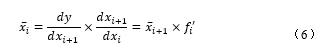In other words, for any function , the derivative of the input  can be determined from the derivative of the output  multiplied by . For ReverseDiff, (3.2) is known as the pullback function, as it pulls the output derivative in backward to calculate the derivative of the input. To evaluate the derivative using the pullback function, we need to know the output derivative and the value of  as well. Thus, a forward evaluation of all the intermediate values must be done and stored first before the reverse differentiation process. Theoretically, the computation time of the ReverseDiff is proportional to the number of outputs, whereas it scales linearly with the number of inputs for ForwardDiff. In practice, ReverseDiff also requires more overhead and memory to store the information during forward calculation. In the examples used in this paper, the input space dimension is on the order of 10³ to 10⁴, but the output space dimension is only 1.

The pullback function is the rule needed to implement for every single operation during the forward calculation. For example, suppose the function we want to evaluate is . Then we need to write a generic pullback function for  as  and for  as .  For the sake of demonstration, we can then combine these two pullback functions as one (will not do in practice as chain rule will take care of) it as:

Notice that the pullback function of the exponent  is known from calculus. However, we can also treat it as a multiplication (a fundamental mathematical operation) of two numbers. The computation graph is shown in Figure 5. The pullback function for multiplication of two real numbers, , is: . Then the pullback function of the input x in Figure 5 is the summation of the two terms in (3.3), which is  when . As can be seen from the example above, any high-level operations can be decomposed into a series of elementary operations such as addition, multiplication, sin(.), and cos(.). Then the pullback function of the high-level operations can always be inferred from the known pullback functions with the chain rule. However, it will be a timesaver if the rules for some high-level operations can be defined directly. Just like the exponent function, it takes much longer computationally to convert it into a series of multiplications, while using a given rule from calculus, such as , is much more efficient. In the structural topology examples demonstrated in Section 4, we will define a custom pullback rule for the backslash operator of the sparse matrix, which results in a much more efficient calculation of the gradient. The implementation details of this rule are discussed in Section 3.2.

3.2. Automatically Differentiate Finite Element Model

A standard forward calculation must be coded as illustrated in the dashed box in Figure 1 to construct a differentiable FEM solver. Then we need to make sure every operation in the forward calculation has a pullback function associated with ReverseDiff. Most elementary mathematical operations in linear algebra have pullback functions well-defined in Julia. However, the operation for solving KU = F, where K is a sparse matrix, has not been defined. Therefore, it is important to write an efficient custom rule for the backslash operator . There are two parts associated with the backslash operation. The first part is to construct a sparse matrix K = sparse(I, J, V ), where I and J are the vectors of row and column indices for non-zero entries and  is a vector of values associated with each entry. The pullback function of the operation is defined as  ( ) = NonZerosOf( ). The process is illustrated in Figure 6. The second part is for the backslash operation. For a symmetric dense matrix, K, the pullback function of  can be written as:

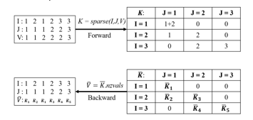Figure 6: Forward and Backward Calculation of sparse(I,J,V) function

The  is the derivative of each element of U with respect to the downstream objective function. In (4.1), it requires two backslash operations, but in practice, the factorization or inverse of K can be reused, and only one expensive factorization is needed. This is why the ReverseDiff can “automatically” calculate the gradient by only evaluating the function in forward mode.

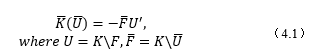When K is sparse, (4.1) can be done efficiently by only using the terms in   and U that correspond to the nonzero entries of the sparse matrix K. Otherwise, (4.1) will result in a dense K matrix that takes up significant memory.

3.3. Programming Language

Julia is used as the programming language. Julia has an excellent ecosystem for scientific computing and automatic differentiation. We use a Julia registered package called ChainRules.jl to define the custom pullback function of the finite element solver. Flux.jl was used to construct the neural network and for optimization.

4. Examples and Results

4.1. 2D Density-based Topology Optimization

Figure 7 is a well-known MBB beam (simply supported beam) for the benchmark test in topology optimization. The objective is to minimize the compliance of the beam subjected to a constant point load applied in the center. Due to symmetry about the vertical axis, the design domain (Figure 7) only includes half of the original problem. The objective function minimizes the displacement at the load point. The equality constraint is that the overall mass fraction of the optimized topology must be consistent with the target mass fraction at the input layer to the generator.

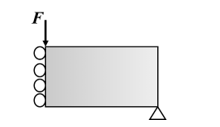Figure 7: Design Domain and Boundary Conditions of MBB Beam

Figure 8 shows the convergence of MBB beam topology design within 100 iterations. The mass fraction is kept as 0.3. It is shown that the objective value in the vertical axis almost flats out at 40 iterations, where the design from the generator stays almost the same afterward.

When assembling the global stiffness matrix  from the element density values, , the actual density value is penalized using , where p ≥ 1. The penalty factor eliminates the checkerboard patterns and creates a smooth boundary. Figure 9 shows side-by-side comparisons of the results from our proposed approach and SIMP 88-line code. The experiment ran combinations of three target mass fraction values and two penalty values for both methods. All designs in Figure 9 are generated after 100 iterations for the MBB beam. The number below each optimized design is the magnitude of the displacement at the applied load point. The proposed method works very well with a low mass fraction design. However, when the mass fraction increases, the details of the design are hard to capture, and a higher penalty value is required to make the design clearer. Although the details of designs from the two methods are different, both methods result in close displacement values. This means the optimized structures have equivalent overall stiffness given the mass fraction, loading, and boundary conditions.

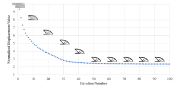Figure 8: Convergence of the Objective Function of the Proposed Method

Table 1 shows the computation time of the proposed method on a 2015 Mac with 2.7GHz Intel i5 Dual Core and 8Gb memory. The time in the table is an average of 100 iterations. The actual time of each iteration varies due to the convergence of the mass constrain in the inner loop as shown in Figure 1.

Table 1: Computation Time of Proposed Method for Each Iteration

Mesh Size	Time (seconds) per Iteration
48*24	0.08
96*48	0.28
192*96	1.3

Figure 10 shows two more cases with different loading and boundary conditions (cantilever beam and bridge) on the density-based topology optimization using the proposed design framework. The cantilever beam on the left has fixed boundary conditions on the left side and a tip load at the midpoint on the right side. The bridge design on the right is simply supported at the lower left and restricted in the vertical direction at lower right. A point load is applied at the midpoint at the bottom surface. The optimized structure using the proposed method does not look exactly like the one using SIMP 88-line code. However, they show similar trends for most of the cases. In Figure 10, the displacement at the applied load point is less using the proposed method, which means the structure has a higher stiffness.

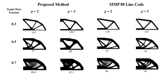Figure 9: Comparisons of Results Between the Proposed Method and 88-line code (Value under each image is the displacement at load point)

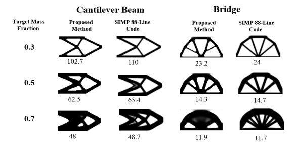Figure 10: Comparisons of Cantilever Beam (Left) and Bridge (Right) Designs using Proposed and SIMP 88-line Method (Value under each image is the displacement at load point)

4.2. 2D Compliant Mechanism Optimization

To demonstrate the flexibility of our proposed method, we use this approach to perform optimization for compliant mechanism design. For a compliant mechanism, the structure must have low compliance at the applied load point but high flexibility at some other part of the structure for desired motion or force output. A force inverter, for example, requires the displacement at point 2 to be in the opposite direction to the applied load at point 1.

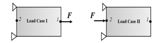Figure 11: Two Load Cases for Optimizing a Compliant Mechanism

Therefore, the objective function has to be formulated as a combination of two parts:

The first term on the right-hand side is the geometry advantage, which is the ratio of the output displacement over input displacement for load case I. This term has to be minimized because the output displacement has to be negative, opposite the input force direction. Also, this term needs to be as negative as possible. However, only this term in the objective function will result in intermediate density and a fragile region around point 2. A second term is added to solve this problem, which measures the compliance of the overall structure, and we want to make sure the structure is stiff when the load is applied at either point 1 or 2. The superscripts  and II denote two different loading cases (Figure 11). For case I, the force is applied at point 1, and displacements are recorded at points 1 and 2. For case II, the force is applied at point 2, and only the displacements at point 2 are recorded. Both displacements at the loading points of the two cases must be minimized to achieve low compliance. Therefore, for each iteration, two load cases, as opposed to one in the previous example, have to be run, and the displacement values will then be fed to the objective functions. The weight coefficient of the second term in (4.2), w, has to be a small number (< 0.1). Otherwise, the design will be too stiff and result in minimal geometry advantage. The image on the left of Figure 12 is the optimized design of this force inverter where w = 0.01 and 0.3 volume ratio. It achieves a geometry advantage of .

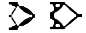Figure 12: Optimized force inverter with different objective functions. Left: use geometry advantage; Right: use target displacement

The geometry advantage in (4.2) can be replaced with . This will make a design with the desired displacement at the output node. The image on the right of Figure12 shows a design with desired target output displacement to be equal to -100. This design is much stiffer at point 2 due to the target displacement (-100) is larger than  -226 of the design on the right of Figure 12. By only the change the objective function, (4.2) ,the proposed method is able to achieve different designs that satisfy the design target.

5. Conclusions

In this work, an integrated physic-informed deep neural network and topology optimization approach is presented as an efficient and flexible way to solve the topology optimization problem. We can calculate the end-to-end gradient information of the entire computational graph by combining the differentiable physics model (FEM) with deep learning layers. The gradient information is used efficiently during the training process of the neural network. We demonstrated the proposed optimization framework on different test cases. Without explicitly specifying any hand-coded equations for gradient calculation and update rules, the neural network after training can learn and produce promising results. The generated optimized structure achieves the same level of overall stiffness as the well-known SIMP method.  The proposed framework is much simpler to implement as only the forward calculations and basic derivative rules are required. For the compliant mechanism design, only the objective function is required to be implemented, and the proposed method can achieve different designs that satisfy the design targets.

6. Declarations

6.1. Funding

No funding was received to assist with this study and the preparation of this manuscript.

6.2. Conflicts of interests/Competing interests

All authors have no conflicts of interest to disclose.

6.3. Availability of data and materials

All data generated or analyzed during the current study are available from the authors on reasonable request.

6.4. Code availability/Replication of results

The data and code will be made available at reader’s request.

1. S.S. Rao, Engineering optimization: theory and practice, John Wiley & Sons, 2019.
2. A. Kentli, “Topology optimization applications on engineering structures,” Truss and Frames—Recent Advances and New Perspectives, 1–23, 2020, doi: 10.5772/intechopen.90474.
3. R.H. Myers, D.C. Montgomery, C.M. Anderson-Cook, Response surface methodology: process and product optimization using designed experiments, John Wiley & Sons, 2016.
4. A.N. Gorban, D.C. Wunsch, “The general approximation theorem,” in 1998 IEEE International Joint Conference on Neural Networks Proceedings. IEEE World Congress on Computational Intelligence (Cat. No.98CH36227), 1271–1274, 1998? doi: 10.1109/ijcnn.1998.685957
5. H. Lin, S. Jegelka, “Resnet with one-neuron hidden layers is a universal approximator,” in Advances in neural information processing systems, 6169–6178, 2018.
6. S. Rawat, M.H. Shen, “A novel topology design approach using an integrated deep learning network architecture,” ArXiv Preprint ArXiv:1808.02334, 2018.
7. M.-H.H. Shen, L. Chen, “A New CGAN Technique for Constrained Topology Design Optimization,” ArXiv Preprint ArXiv:1901.07675, 2019.
8. Z. Nie, T. Lin, H. Jiang, L.B. Kara, “Topologygan: Topology optimization using generative adversarial networks based on physical fields over the initial domain,” Journal of Mechanical Design, 143(3), 31715, 2021, doi: 10.1115/1.4049533
9. W. Chen, K. Chiu, M.D. Fuge, “Airfoil Design Parameterization and Optimization Using Bézier Generative Adversarial Networks,” AIAA Journal, 58(11), 4723–4735, 2020, doi: 10.2514/1.j059317
10. M. Innes, A. Edelman, K. Fischer, C. Rackauckus, E. Saba, V.B. Shah, W. Tebbutt, “Zygote: A differentiable programming system to bridge machine learning and scientific computing,” ArXiv Preprint ArXiv:1907.07587, 140, 2019.
11. M. Innes, “Don’t unroll adjoint: differentiating SSA-Form programs,” ArXiv Preprint ArXiv:1810.07951, 2018.
12. S.A. Nørgaard, M. Sagebaum, N.R. Gauger, B.S. Lazarov, “Applications of automatic differentiation in topology optimization,” Structural and Multidisciplinary Optimization, 56(5), 1135–1146, 2017, doi: 10.1007/s00158-017-1708-2
13. S.B. Dilgen, C.B. Dilgen, D.R. Fuhrman, O. Sigmund, B.S. Lazarov, “Density based topology optimization of turbulent flow heat transfer systems,” Structural and Multidisciplinary Optimization, 57(5), 1905–1918, 2018, doi: 10.1007/s00158-018-1967-6
14. A. Vadakkepatt, S.R. Mathur, J.Y. Murthy, “Efficient automatic discrete adjoint sensitivity computation for topology optimization–heat conduction applications,” International Journal of Numerical Methods for Heat & Fluid Flow, 2018, doi: 10.1108/hff-01-2017-0011
15. M. Raissi, P. Perdikaris, G.E. Karniadakis, “Physics-informed neural networks: A deep learning framework for solving forward and inverse problems involving nonlinear partial differential equations,” Journal of Computational Physics, 378, 686–707, 2019, doi: 10.1016/j.jcp.2018.10.045
16. Z. Mao, A.D. Jagtap, G.E. Karniadakis, “Physics-informed neural networks for high-speed flows,” Computer Methods in Applied Mechanics and Engineering, 360, 112789, 2020, doi: 10.1016/j.cma.2019.112789
17. X.I.A. Yang, S. Zafar, J.-X. Wang, H. Xiao, “Predictive large-eddy-simulation wall modeling via physics-informed neural networks,” Physical Review Fluids, 4(3), 34602, 2019, doi: 10.1103/physrevfluids.4.034602
18. X. Jin, S. Cai, H. Li, G.E. Karniadakis, “NSFnets (Navier-Stokes flow nets): Physics-informed neural networks for the incompressible Navier-Stokes equations,” Journal of Computational Physics, 426, 109951, 2021, doi: 10.1016/j.jcp.2020.109951
19. M.P. Bendsoe, O. Sigmund, Topology optimization: theory, methods, and applications, Springer Science & Business Media, 2013.
20. G. Allaire, “A review of adjoint methods for sensitivity analysis, uncertainty quantification and optimization in numerical codes,” 2015.
21. M.Y. Wang, X. Wang, D. Guo, “A level set method for structural topology optimization,” Computer Methods in Applied Mechanics and Engineering, 192(1–2), 227–246, 2003.
22. X.Y. Yang, Y.M. Xie, G.P. Steven, O.M. Querin, “Bidirectional evolutionary method for stiffness optimization,” AIAA Journal, 37(11), 1483–1488, 1999,doi: 10.2514/2.626
23. D.P. Kingma, J. Ba, “Adam: A method for stochastic optimization,” ArXiv Preprint ArXiv:1412.6980, 2014.
24. I. Goodfellow, J. Pouget-Abadie, M. Mirza, B. Xu, D. Warde-Farley, S. Ozair, A. Courville, Y. Bengio, “Generative adversarial nets,” in Advances in neural information processing systems, 2672–2680, 2014.
25. E. Andreassen, A. Clausen, M. Schevenels, B.S. Lazarov, O. Sigmund, “Efficient topology optimization in MATLAB using 88 lines of code,” Structural and Multidisciplinary Optimization, 43(1), 1–16, 2011, doi: Andreassen_2010
26. B. Bourdin, “Filters in topology optimization,” International Journal for Numerical Methods in Engineering, 50(9), 2143–2158, 2001, doi: 10.1002/nme.116
27. J. Revels, M. Lubin, T. Papamarkou, “Forward-mode automatic differentiation in Julia,” ArXiv Preprint ArXiv:1607.07892, 2016.
28. G. Allaire, F. Jouve, A.-M. Toader, “Structural optimization using sensitivity analysis and a level-set method,” Journal of Computational Physics, 194(1), 363–393, 2004,doi: 10.1016/j.jcp.2003.09.032
29. R.M. Errico, “What is an adjoint model?,” Bulletin of the American Meteorological Society, 78(11), 2577–2592, 1997.
30. M.A. Akgun, R.T. Haftka, K.C. Wu, J.L. Walsh, J.H. Garcelon, “Efficient structural optimization for multiple load cases using adjoint sensitivities,” AIAA Journal, 39(3), 511–516, 2001,doi: 10.2514/3.14760
31. R.T. Haftka, Z. Gürdal, Elements of structural optimization, Springer Science & Business Media, 2012.
32. R. Hecht-Nielsen, Theory of the backpropagation neural network, Elsevier: 65–93, 1992, doi: 10.1109/ijcnn.1989.118638

(Click Here)