1. Introduction

Automatic speech recognition (ASR) is still an intriguing and demanding subject among researchers around the world. It is the mechanism that enables human-machine interaction through speech orders.  In the present of the Coronavirus outbreak, this technology could decrease the propagation of the infection because no physical interaction such as touchscreen is required. Moreover, the automatic speech recognition system could also provide the hand-free experience that produces the huge advantage among the handicapped and visually impaired people.  This manuscript is an extension of work that was initially presented in the 2021 Second International Symposium on Instrumentation, Control, Artificial Intelligence, and Robotics (ICA-SYMP) [1]. In Thailand, according to the computers and the Thai language research [2], the first development of Thai ASR system concerned about isolated word recognition, which could be used for short commands [3]. The other improved method, which might be employed for continuous voice in little jobs, such as e-mail access or telephone banking, was also offered. More researches were publishing on huge vocabulary continuous speech recognition, or LVCSR [4], [5]. Inadequate speech databases and Thai-language complexity such as letter-to-sound mapping, phoneme set selection, segmentation, and tonality, were the key problems when developed a Thai automatic speech recognition system as mentioned in [6]. Nevertheless, many Thai organizations put effort in developing Thai speech corpus such as the LOTUS corpus by NECTEC [7].  For the standard automatic speech recognition system in natural language processing (NLP), it consisted of three basic models: Acoustic model, Lexicon, and Language model. For Thai language, the limitation of available large speech database and the complexity of Thai language could contribute to delayed speech recognition improvement [2].

      In an effort to solve the problem, the automatic speech recognition was constructed using the different approach. The proposed method used the keyword spotting methodology to recognize the Thai sentence linked to the categorized keywords instead of using the traditional ASR system. This approach could ignore the presence of unpredictable words in the utterances such as unprecedented words and non-speech sounds. In such a case, the typical method must include the large vocabularies, as well as grammars.

More details about the keyword spotting were clearly mentioned in the following section. For investigating more corresponding Thai research, the use of acoustic modeling based on Hidden Markov Models (HMMs) method [8], [9]. The models consisted of filler models, syllable models, and keyword models, which used for handling out-of-vocabulary sound elements in the speech recognition using the keyword spotting algorithm. Another paper proposed the nondestructive determination of maturity of the Monthong Durian based on Mel-Frequency Ceptral Coefficients (MFCCs) and Neural Network. Then we have further investigated more excellent works that related to ours like SpeechYOLO paper [10], this paper used first version of YOLO with keyword spotting algorithm for localizing boundaries of utterances within input signal by considering audio as objects and use Short-Time Fourier Transform (STFT) technique to extract the audio feature. In our research we have identified a similar approach in order to solve the limitations in Thai speech recognition field, but we use the improved version of YOLO which was YOLOv3 and we also use Mel-Frequency Cepstral Coefficients (MFCC) technique which could artificially implement the behavior of the human auditory perception due to the fact that it is capable of using the non-linear Mel scale which relies on the non-linear frequency scale of the real human.

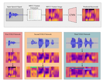Figure 1: Top: the core methodology pipeline composed of the Mel-Frequency Cepstral Coefficient (MFCC) as the feature extraction method and the YOLOv3 as the popular convolutional neural network (CNN) based object detector which was then applied to localize and classify keywords. Bottom: our proposed method for the real-world application, which consisted of three separated YOLO networks including airline names, numbers (0-9), and frequently asked questions (FAQs). Both full and tiny version of YOLOv3 were proposed.

      This manuscript started with explaining how Keyword Spotting (KWS) to clarify the speaker propose and also investigated the KWS prior works. Then, the system pipeline will be explained which started from the speech feature analysis extraction method. This process was crucial since it could represent the voice signal information in the form of a feature image. Consequently, in the next section, the convolutional neural network was explained including the history of object detection techniques, the novel CNN-based object detectors, and the major improvement in YOLO family. After that, the voice dataset collection is described. Then, the highlights of our core methodology are explained. This manuscript also explained about the YOLO annotation and network training. Finally, the proposed method consisted of three networks was experimented. These three networks were responsible for three real-world tasks that would then introduce in the following section. In the last section of this manuscript, the comparison between the regular and the light-weight version of YOLOv3 performances was discussed for the additional usage in the low-resource platform.    The overall design of our work was displayed in Figure 1.

2. Keyword Spotting for the Spoken Sentence

In general, most people tend to struggle to understand the spoken sentences especially with the native speakers. Unlike a written sentence, the spoken sentence is more difficult and variety in terms of speed, accent, style, or tone depending on the morphological richness of each language such as Thai language as previously mentioned. The most reasonable answer why the spoken sentence is difficult is that we don’t experience enough vocabularies. Many scientists also say that listening requires more vocabulary knowledge than reading. In addition, it is difficult to tell whether the sentence contains unknown terms or is quickly spoken. Eventually, the spoken words are not always finished or carefully delivered with the native speakers like syllable stressing or skipping some words. Just like the human, the machine must transcribe the entire sentence with a huge model of vocabulary. To address this issue, the keywords are employed to involve the main idea rather than to use every single word in the sentence. This idea was motivated by the scanning strategies used in the reading comprehension test. Many skillful readers used this technique to reduce time to search for some specific information by just looking for the related words instead of reading the whole paragraph line by line. This scanning technique also seemed to help the system to come across the complexity and the variety of the sentence structures.

       For the ASR system, there were certain technologies known as wake word, the particular word or phrase which would enable some additional functions. These voice-related systems, such as “Hey Siri” by Apple’s Siri or “OK Google” by Google Now, exploited the keyword spotting (KWS) method which would listen until the specific keywords could be recognized [11]. The prior work for KWS introduced the Keyword/Filler Hidden Markov Model (HMM) [12]. Each keyword was trained with the HMM model, then the non-keyword segments, so-called fillers, was trained separately with a filler model HMM. Due to the decoding need of Viterbi, this strategy ended with considerable computational complexity. Then, the following enhanced approaches concerned the use of the discriminative model on the keyword spotting task, namely, large-margin formulation [13] and recurrent neural networks [14]. Although it could produce many significant improvements over the traditional HMM method, the high computational time was still occurred due to the entire utterance processing in order to locate an optimal area of keywords. These limitations were still challenging until Google proposed the novel deep learning keyword spotting approach base on the deep neural network, also called DeepKWS. Since this method could provide high detection performance with smaller memory consumption and shorter runtime computation, then it was appropriate for the mobile device usage. Unlike the HMM approach, this process did not require the excessive sequence search algorithm. After that, Google explored a small-footprint keyword spotting (KWS) system using the Convolutional Neural Networks (CNNs) [15]. The CNN approach could outperform the DeepKWS in many ways. For instance, it provided more robustness over different speaking styles, reduced model size and more practical for spectral representation input. Thus, in this research, we chose the CNN-based object detection for localizing and classify Thai keywords from the spoken sentence.

3. Speech Feature Analysis and Extraction

Automatic Speech Recognition (ASR) system is influenced by feature analysis and extraction, since the high-quality features provide an acceptable and dependable results in the localization and classification process. The main purpose of feature extraction is to reveal acoustic information in terms of a sequence of feature vectors, which can successfully characterize a given speech data. Several feature extraction techniques are available to extract the parametric representation of the audio signal, such as perceptual linear prediction (PLP), linear prediction coding (LPC) and Mel-frequency Cepstral Coefficients (MFCC). MFCC has been proven to be the most prevalent and powerful technique [16], [17].

      Mel-Frequency Cepstral Coefficients (MFCC) is the transformation from the speech waveform to frequency domain mathematical features, which are considered to be much more accurate than time domain features. This technique artificially implements the behavior of the human auditory perception due to the fact that it uses the non-linear Mel scale which relies on the non-linear frequency scale of the real human, so it results in the parametrically resemblances between the extracted vectors and human sense of hearing. The output of the MFCC is a short-term power spectrum coefficient of a windowed signal produced from the original signal Fast Fourier Transform (FFT). This transformation is done using the logarithmic power spectrum through a linear transformation, Discrete Cosine Transform (DCT). MFCC for speech can reveal more compact spectrum since Mel-scale coefficients are countable.

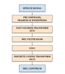Figure 2: The overall MFCC derivation

      In detail, the overall MFCC feature extraction technique is shown in Figure 2. It consists of windowing the speech signal, applying the Fast Fourier Transform (FFT), taking the log of the magnitude, warping the frequencies on a Mel scale, applying the Discrete Cosine Transform (DCT). In order to remove the MFCC from the speech signal, pre-emphasis begins. Compensate filtering for the high frequency area disappearing during the mechanism of voice creation are considered in the pre-emphasis. In addition, the significant of the high-frequency component is also strengthened. This step is therefore followed by the high-pass filter as explained in (1).

where,

       is the input signal.

       is the output signal.

       is a control slope of the filter ranged from 0.9 to 1.0

The z-transform of the filter is defined as (2).

After the pre-emphasis process, the spectrum of the signal is balanced and some glottal effects from the vocal tract parameters are removed. Then the speech signal needs to be analyzed over a short period of time by capturing into a discrete frame, with some overlapping between frames. The purpose of the overlapping analysis is to approximately center each speech signal at some frame and avoid significant information loss. On each frame, the Hamming window is multiplied individually to maintain the continuity of the first and the last points in a frame. If the signal in a frame is denoted by  then the signal after windowing is applied will be where represented the Hamming windowing defined as (3)

where,

       is the Hamming window.

      is the total number of samples in a frame.

      is a sample number.

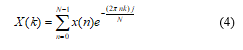
Each short-time frame was then transformed into the spectral features by applying the Fast Fourier Transform (FFT), which was the accelerated version of the Discrete Fourier Transform (DFT). This technique converted each frame of  samples from the time domain into frequency domain and was shown in (4).

where,

       is the total number of points in the FFT computation.

Next, the Fourier transformed output was passed through a set of band-pass filters, so called Logarithmic Mel-filter bank, in order to cover from a real frequency, estimated in the Hertz unit, , into the Mel unit, , by the equation (5). The Mel scale was about a linear frequency spacing of less than 1 kHz and a logarithmic spacing of more than 1 kHz, respectively.

The frequency of Mel-scale is proportional to the linear frequency logarithm. Due to the fact that the behavior of human’s aural perception is non-linear, this concept can be implemented using Mel-scale filter bank, which is commonly the combination of the K triangular filters. The example of a filter bank with K=20 is illustrated in Figure 3.  The higher frequency filters contain more bandwidth than the lower frequency filters, but they share similar temporal constraints. Each triangular filter is centered with a maximum amplitude of 1 and is reduced linearly to zero until it approaches the central frequency of the two neighboring filters, where zero response is present and can be derived as (6).

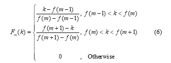
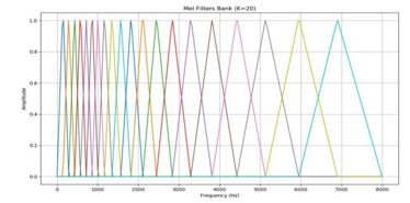Figure 3: Mel filters bank when K=20

where,

       is the filter number  at  frequency.

       is the filter number in Mel filters bank.

Therefore, the Mel spectrum of the frequency spectrum  was calculated by multiplying the spectrum by each of the triangular Mel weighting filters as shown in (7).

where,

         is the total number of triangular Mel weighting filters.

      The Discrete Cosine Transformation (DCT) was then applied on the transformed Mel frequency coefficients in order to produce a set of twelve cepstral coefficients. Since this algorithm, which was described in (8), resulted in a signal with a quefrency peak in the time-like domain, so called cepstral domain. Thus, Mel-Frequency Cepstral Coefficients, or MFCC, was nominated from the final features which were similar to cepstrum. The zeroth coefficient was excluded because it contained the unreliable information.

where,

        is the frequency coefficient.

        is the cepstral coefficient.

         is the number of MFCCs.

        is the number of triangular bandpass filters.

      Following this phase, a speech signal in the form of an MFCC might be employed to perform machine learning technology or treated as an ordinary image. The MFCC for each speech frame was stacked and converted into an RGB image with Plasma color map. Figure 4 shows examples of MFCC’s Thai keyword images which include check-in, price and what time is it respectively.

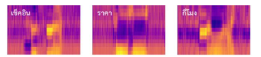Figure 4: The examples of Thai keyword MFCCs

4. Convolutional Neural Networks for Voice Image

The sequence of the cepstral vectors or MFCC characteristics was received from the recorded voice as an input as previously discussed in the last section. The next step is to derive the corresponding keywords. In this section, computer vision technique for the Natural Language Processing (NLP) task is detailed. In order to resolve this challenge, we opted to employ a state-of-the-art object detection algorithm because it can be used to estimate the location (object localization) and category (object classification) of each object in a given image. Therefore, this technique should be able to extract the important sort of information for better semantic understanding of images [18]. From the preceding progress, as a result of considering MFCC features as the normal image, then keywords can be comparative to objects. Thus, the object detection is well-suited and also helpful for solving this situation as shown in Figure 5. The object detection technique that we chose in our work is the novel deep learning approach based on Convolutional neural network (CNN) [18][19]. CNN is a specialized type of neural network model modified especially for dealing with two-dimensional input data.

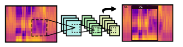Figure 5: Object detection on MFCCs.

It is typically composed of three fundamental types of layer consisting of convolutional, pooling and fully connected layers. Convolutional and pooling layers contain filters, whose depth increases from left to right while width and height have the inverse proportion, have an interactive role in extracting features. The Convolutional layer is denominated from the important linear mathematical operation in the layer, so-called convolution, or filtering. The convolution function is described in (9).

where,

       is the two-dimensional array such as Image.

       is filter or kernel.

      is the output or feature map.

This operation involves the dot product between the input array and the filter or kernel, by convolving across its width and height, then extended throughout its depth. Next, the result from convolution is passed through an activation unit called Rectified Linear Unit (ReLU) calculated by (10). It is a piecewise function that will return the input directly if the input value is positive, otherwise, it will return zero.

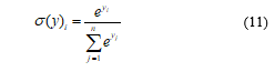
Subsequently, it is down sampled or normalized by the pooling operation, e.g. max pooling, in the pooling layer. This operation summarizes the initial activation feature map to become more robust. After that, fully connected layers then map them into output via activation function, which normally uses the Softmax activation defined in (11). It provides the probability distribution for each neuron, in the same way as a traditional neural network.

where,

       are the element of the input vector.

       is the total number of classes.

        is the input vector.

The learning parameters can be optimized via the Stochastic gradient descent (SGD) method and the back propagation, called the training, in each layer across the models. The algorithms aim to minimize the difference between prediction and ground truth. Therefore, in the training process, the dataset images are fed forward with initial kernels and weights, so-called forward propagation. Then a model’s accuracy is calculated by a loss function. The error value is used for updating kernels and weights later in the back propagation using gradient descent optimization. The overview of convolutional neural network architecture and the parameter optimization process are illustrated in Figure 6.

      The convolutional neural network has been shown to be outperformed to previous methodologies in many ways. Firstly, Spatial Hierarchical feature representation can be learned automatically and the multiple nonlinear mappings can reveal the hidden patterns. Then deeper architecture, which significantly increases the model competency, allows related task optimization. Finally, due to the uprising of CNN learning performance, some challenging computer vision problems might be solved from a new perspective. CNN method has also been popular among various research topics such as facial recognition [22] and pedestrian detection [23]. CNN-based object detection technique aims to identify the location and the class of every object existing in the input image. Nowadays, its frameworks can be divided into two main categories, which are two-stage and one-stage approaches. A two-stage model is a technique that is constructed based on the standard object detection pipeline. It proposes two separate consecutive methods which are region proposal and object classification. In detail, region proposals are generated first, then each proposal will be classified according to the object classes. The second methodology, which is a one-stage model, considers transforming the traditional object detection problem to the regression problem by merging all separated tasks, consisting of localization and classification, into a single unified model.

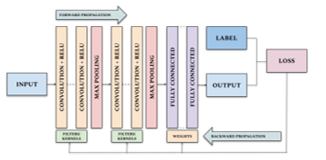Figure 6: CNN architecture and the training process.

      For the two-stage method, in [22], the author introduced the proposal of the regions with CNN features (R-CNN), which took a giant step towards object detection. It extracts a set of object candidate boxes or proposals by using a selective search method, which leads to major improvement in detection accuracy. However, this technique experiences many drawbacks. The enormous quantities of overlapped repetition boxes greatly delay the overall process and some feature losses can also be due to proposals in fixed candidate region. To solve the problems, in [23], the author proposed Spatial Pyramid Pooling Networks (SPPNet). The Spatial Pyramid Pooling (SPP) layer in SPPNet allows a CNN to construct a representation without considering the input image size. Although SPPNet utilizes less processing time than R-CNN since it requires only the single computing for the convolutional layer, the downside of this approach is the extended training period and the high use of disk space.  The several advantages from R-CNN and SPPNet were investigated and integrated in the following work, Fast RCNN, but the detection speed is still bounded by the selective search [24]. Therefore, in [25], the author proposed Faster RCNN, which was known as the first ever end-to-end object detector that could almost yield real-time performance. It can break through the speed bottleneck of past efforts by demonstrating the use of the region proposal networks (RPN) instead of the traditional selective search method. In addition, it uses a separate network to predict the region proposals only. The region proposal network is trained together with the model which results in predicting more accurate proposed regions. Later, there were some further improvement efforts on Faster RCNN, such as Feature Pyramid Networks (FPN) introduced in [26]. With the small object constraints, a basic image pyramid can be used to scale input images into multiple sizes before sending to the network. The FPN has enhanced the performance of multi-scale object detection and has become a model for numerous novel approaches.

      On the one hand, the two-stage detector comes up with high localization and classification accuracy. On the other hand, its inference speed is impractical for the real-time applications, especially for the low-resource computational platforms like embedded systems, and the complex procedures of its core methodology could possibly diminish the opportunities of further optimization and improvement over components. The one-stage models have been built and researched in order to overcome these restrictions. It recognized objects based on two distinct neural networks, which lead to high computational time as indicated before in Faster RCNN section. Accordingly, the one-stage method combines feature extraction, region proposal and object classification altogether into a single network. The object classification is also performed regarding the predefined size and number of anchor boxes specified in the model configuration, then the regression concept is applied for the object localization process. Consequently, this novel breakthrough could implement the object detection as a single regression problem by predicting bounding box coordination and class probability simultaneously. The one-stage object detection pipeline used in our work is shown in Figure 7.

Figure 7: The basic architecture of one-stage object detector using MFCC voice image as the model input.

      The one-stage object detectors were demonstrated to attract a great deal of attention amongst researchers not only because they can overcome the problem of a real-time bottleneck in the two-stage approaches, but because it could generate similar detection performance, it the detection speed and accuracy trade-off is well-optimized. Since our application is based on the Automatic Speech Recognition (ASR), both processing time and detection performance must be concerned. Therefore, we have chosen the state-of-the-art one-stage approach called YOLO, which is You Only Look Once. Based on real-time criteria, the computational time must be considered more than 10 frames per second (FPS) or less than 100 milliseconds. The performance evaluation results published in the YOLO article meet our requirements and stated that the third version of YOLO, or YOLOv3, outperforms other popular methods such as Single Shot Multibox Detector (SSD) [27], which had the original implementation on Caffe [28].

      You Only Look Once (YOLO) is the prominent one-stage CNN-based object detector which we have chosen as a Thai keyword localizer and classifier in our research due to the high calculation speed and acceptable detection accuracy on the real-time task. YOLO frames object detection as a regression problem, thus it can simultaneously construct the object bounding boxes and predict class probabilities, while it needs only one forward propagation from the input image. The model name, You Only Look Once, might therefore be designated from such properties.

      YOLO divides the input image into  grid. Then, each grid cell takes responsibility for detecting the object whenever its center approaches that particular grid cell boundary. Each grid cell will predict bounding boxes and their predicted confidence scores. The bounding boxes can be represented by five parameters including  and the confidence scores. The parameters  indicate the center coordination of the box relative to the grid cell area. The next two parameters  describe the width and height of the box relative to overall image dimensions. The last parameter, the confidence scores can be derived from (12).

where,

   tells how likely the object existence is.

   tells how accurate the predicted box is.

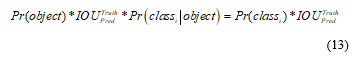
At that moment, each grid cell also predicts   conditional class probabilities, which is the conditional probabilities of the grid cell detecting an object, regardless of the number of boxes. The prediction is finally encoded as a  tensor and the final confident scores can be described by Equation (13).

where,

          is the conditional class probability.

During the model training step, the loss function is optimized and could be described in (14). From the following equation, we can notice that the loss function only penalizes the classification errors when an object exists in that corresponding grid cell, and likewise, the errors of the bounding box coordinate are penalized when a prediction is literally responsible for the ground truth.

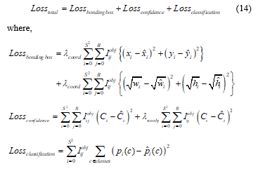where,

In the first version of YOLO [28], the network architecture was designed based on the GoogLeNet[29] architecture for image classification. YOLOv1 network consists of 24 convolutional layers and 2 fully connected layers. It replaced GoogLeNet’s inception modules with 1 x 1 reduction layers and 3 x 3 convolutional layers respectively.  The first 20 convolutional layers of the network were pretrained on the classic ImageNet 1000-class competition dataset with the input size of 244 x 244 to have 88% top-5 accuracy for a week. The PASCAL Visual Object Classes (VOC) in 2007 and 2012 were then used for training and validation. On this dataset, 98 bounding boxes per images are predicted. The weak predictions are then filtered out by the Non-maximum Suppression (NMS) technique. The overall training pipeline was originally implemented on the Darknet framework. YOLOv1 could achieve 63.4 mAP (mean average precision) and 45 FPS (frames per second). This achievement implicated that YOLO could perform real-time performance while the detection accuracy was as comparable as Faster R-CNN. To improve YOLO’s detection speed, Fast YOLO was introduced [30]. It optimized the original YOLO architecture by decreasing the convolutional layers from 24 to 9 and using fewer filters in those layers. Therefore, it could reach up to 155 FPS, but the accuracy dropped to 52.7% mAP.

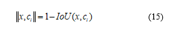
      For considering the generalizability, YOLOv1 performed well on PASCAL VOC 2007 and it seemed to be the best method when evaluated on the artwork dataset which contained the challenging difficulty on a pixel level. Although YOLOv1 could achieve significant achievement over other methods, it also struggled with some limitations. Since the classification and localization network of this version of YOLO could detect only one object, any grid cell could detect one object too. This constraint resulted in the limit maximum number of objects, which was a total of 49 objects per one detection for 7×7 grid cells. As a result, it caused relatively high localization error especially the small objects that close to each other, such as groups of pedestrians. Moreover, this network architecture found difficulty in object generalization when evaluating on the other input dimensions instead of 244 x 244. To overcome these YOLOv1 constraints and achieve better performance, the second version of YOLO (YOLOv2) was then developed [31]. YOLOv2 concerned mainly about maintaining the prior classification performance while it also worked on improving recall and localization. Thus, it applied a variety of significant modifications to increase mean average precision (mAP). By adding batch normalization on the convolution layers, the model showed drastic impact on the convergence. In detail, the activations in the hidden layer were shifting and scaling which leaded to improving model stability and also reducing the overfitting issue. This technique could raise YOLO’s mAP up to 2% and has been widely used for the model regularization propose. Consequently, YOLOv2 also proposed the high-resolution classifier from 224×244 in the first version to 448×448. Initially, the model was trained on the 224×224 input images, then the classification network was fine-tuned with 448×448 resolution on the ImageNet dataset for 10 epochs before detection training. This process gave a room for kernel adjustment on higher resolution images, which therefore resulted in better detection performance and reached slightly below 4% mAP improvement. Moreover, YOLOv2’s researcher has introduced the remarkable progress, motivated by Faster R-CNN, which was the usage of anchor box. Instead of using fully-connected layers for bounding box prediction on the feature map, the convolutional layers were modified to predict locations of anchor boxes which leaded to recall increasing, but slightly degraded the overall mAP. The bounding box prediction could then relative to these anchor boxes, which was a small area consisted of width and height, unlike in YOLOv1 that relative to full image dimension. As mentioned in Faster R-CNN, the initial sizes of anchor boxes were chosen by hand-picking method. In contrast, YOLOv2 developer designed the suitable anchor box dimensions using k-mean clustering. The distance metric was calculated based on IoU scores, which is shown in (15).

where,

         is a ground truth candidate box.

         is one of the centroids.

The YOLOv2 bounding box prediction spatially related to the offsets of the anchors. It predicted 5 parameters including tx, ty, tw, th and to, then applied the sigma function to limit the offset range of an output, which was calculated by (16).

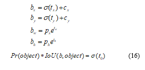where,

          are the predicted offset and scale.

        are the top left corner of the anchor grid cell.

         are the size of the anchor box.

         are the predicted box center and size.

        is the box confidence score.

These anchor boxes generated by clustering technique could provide higher average IoU. YOLOv2 divided the input into 13×13 grid cells by removing a pooling layer that was later more helpful with larger or smaller items. The goal was also to overcome a small object limitation in YOLOv1. Furthermore, this version of YOLO model also integrated the multi-scale training strategy that could strengthen the model robustness to various input image sizes. Every 10 batches during training process, the network was resized according to the new random image dimension which was a multiple of 32 dues to convolutional layer down sampling property. Lastly, for reducing the computation time, YOLOv2 used a more light-weighted base model architecture, so called Darknet-19, with 19 convolutional layers and 5 layers of max-pooling. In addition, YOLOv2 also had the extended version which could detect more than 9000 classes, also known as YOLO9000 [31]. YOLO9000 was a slightly modified version of YOLOv2, which considered in merging small object detection dataset with large ImageNet dataset. Since the overlapping class labels of these two datasets could not combine directly, the WordTree hierarchical model was demonstrated for this difficulty. The general labels were placed in the top closer to the root and the fine-grained labels were branched similar to leaves. The probability of each class could calculate by following the path from that node to the root.

      YOLOv3 was another improved version of YOLO family which outperformed its predecessor by using the state-of-the-art algorithms and also was practical with real-time scenarios [32]. Firstly, in order to predict the objectness confidence score, YOLOv3 proposed the logistic regression for predicting the confidence score for each bounding box, while the prior YOLOs used the sum of the square errors. Next, in some dataset like ImageNet, not all the labels were mutually exclusive. In such a case, choosing the Softmax function as the activation function of the output layer might not be the best choice, since it just converted predicted scores to distributed probabilities which summed up to one. For instead, YOLOv3 used multiple independent logistic classifier. The input image could then have multiple labels and contained both mutually and non-mutually exclusive objects. The complexity of the YOLOv3 model was also decreased by getting rid of the Softmax function. Consequently, with the new activation functions, the classification loss function must be modified into the binary cross-entropy instead of the Mean Square Error (MSE). Inspired by the idea of the Feature Pyramid Network (FPN), YOLOv3 could then predict the object up to three different box scales for every location in the input image and then perform feature extraction. This technique improved the detection performance on various object scales and was a significant solution especially for detecting small things. The Feature Pyramid Network design was illustrated in Figure 8.  Furthermore, YOLOv3 also adopted cross-layer connections between two prediction layers and the fine-grained feature maps. Initially, the coarse-grained feature map was up-sampled, then the concatenation was performed to combine it with the previous one. Moreover, the YOLO’s feature extractor was modified from Darknet-19 to Darknet-53, which based on the 53 convolutional layers. Darknet-53 was much deeper and composed of mostly 3×3 and 1×1 kernels including skip connections just like residual network in ResNet. In comparison, it has less BFLOP (billion floating point operations) than ResNet-152, but could still maintain the same detection accuracy at two-times faster. The full YOLOv3 architecture was illustrated in Figure 9.

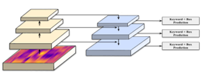Figure 8:  Feature Pyramid Network.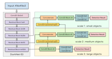Figure 9:  The YOLOv3 architecture.

YOLOv3 may therefore conduct high-detection capabilities for object detecion. In YOLOv3 paper, the researcher argued that YOLOv3 might exceed three times the speed of the Single Shot Multibox Detector (SSD). While RetinaNet was more precise, it also battled with the computational time. In small object criteria, YOLOv3 has also shown substantial progress.

      YOLOv3 also had the lightweight version which was known as the tiny-YOLOv3 model. It used the same training strategy as the full version, however, the minor modifications were applied with the full YOLOv3 model architecture to gain a lot more computation speed and consume fewer computational resources for inference. This model was ideally optimized for the use of the low resource platform such as embedded systems and mobile devices. Firstly, the tiny-YOLOv3 simplified the number of convolutional layers. It used only 7 convolutional layers. This tiny version just employed a few numbers of 1×1 and 3×3 convolutional layers for extraction of features. It replaced a convolution layer with the pooling layer with a step size of 2 by focusing on summarized the complex dimension of the standard model. Although it used a slightly different architecture with the full YOLOv3, the model base structure was still the same which composed of 2D-convolutional, batch normalization and Leaky Rectified Linear Unit (ReLU).

      In our research, the speech signal can now be handled as an ordinary image by transforming the recorded voice signal into the MFCC feature image. Then, Thai spoken keywords that contain with in the voice image could be compared as objects. Therefore, the object detection technique could be applied to an automatic speech recognition task. In order to understand the Thai speaker purpose, we applied this core methodology to find the corresponding Thai keywords in the voice image by feeding the whole sentence MFCC and matched them with our predefined sentence categories which each group of Thai keywords related to. Moreover, we propose that the localization ability of the object detector could be deployed especially with some input spoken sentence, which relies on the restricted keyword ordering such as the unique number sequence in the flight number. As mentioned previously, YOLOv3 has been proven to be fast and accurate. It was the most stable and reliable version of YOLO since we started to research this work. We also compared the detection performance between the full-YOLOv3 and its tiny version. Since tiny-YOLOv3 was extremely fast, some mean average precision (mAP) was traded off. Our keyword detection system was illustrated in Figure 10.

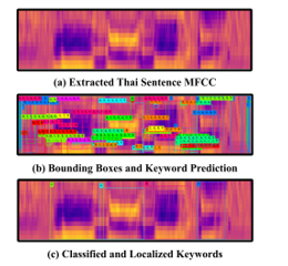Figure 10: The keyword detection overview with Thai sentence MFCC feature image as an input.

5. Voice Dataset Collecting and Preprocessing

This article draws on speech datasets made by 60 native Thai speakers and recorded in several places proposed to simulate the variety of the background noises. Our selected participants were varied in ages and the genders were equally distributed. In terms of age, the highest number of overall participated subjects was in teenage (20s), which was 18 people (30%), and those aged between 40 and 49 were the smallest, which was 7 people (11.6%). The total datasets contained 2400 WAV files with 40 unique keywords. Table 1 summarized the baseline characteristic of our dataset. At the beginning, each recorded voice was processed using the Audacity software before converting into MFCC feature image, which was shown in Figure 11 and 12.

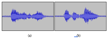Figure 11: The examples of recorded voice: (a) แอร์เอเชีย (Air Asia);  (b)  การบินไทย (Thai Airways)

In order to avoid overfitting and improve the model robustness, some data augmentation methods including the tempo and pitch randomizing were applied to increase the quantity of training data, therefore finally finishing up with a total of 9600 WAV files. The datasets were obtained in accordance with the passenger information machine criteria for the research of the automatic speech recognition (ASR) system in actual settings. The automated system required to give the reliable information, which correlate to the passenger’s flight number as a real-time answer to the passenger’s frequently asked questions (FAQs). In the aviation industry, a flight number is composed of a two-character airline designator and numbers with a maximum length of four digits. Thus, we proposed three datasets consisted of airline names, numbers and FAQs keywords. The first dataset was selected from the ten popular airlines at the Suvarnabhumi airport in Thailand. Next, the second dataset consisted of ten numbers (0-9). The final dataset contained 20 keywords which could categorize into 7 passenger FAQ topics.

Table 1: The baseline characteristic of our dataset.

Characteristics	Training (80%)	Validation (20%)	Total
Population	48	12	60
Sex
Male	24	6	30
Female	24	6	30
Age Group (Y)
10-19	9	2	11
20-29	15	3	18
30-39	6	2	8
40-49	6	1	7
50-59	6	2	8
60-69	6	2	8
.WAV files
Raw Dataset	1920	480	2400
Raw Dataset + Augmentation	7680	1920	9600

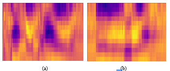Figure 12: The examples of extracted MFCC image: (a) แอร์เอเชีย (Air Asia);  (b)  การบินไทย (Thai Airways).

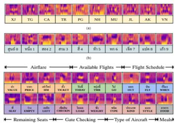Figure 13: The overview of three datasets: (a) airline designators; (b) numbers 0-9; (c) FAQs keywords

      Figure 13 showed the overview of three datasets.  In every dataset, the images were randomly split with a ratio of 80:10:10, which included training, validation, and also test sets for further evaluation.

6. Highlights of the Research Work

In Thai linguistics, the absence of large speech corpora and the language morphology could inhibit development and researches in the speech recognition field as mentioned on the introduction section. Although several organizations like NEXTEC concentrated on eliminating this limitation, the complicity of the spontaneous voice input, especially in a noisy environment, seemed to be a problem for many researchers. Through the keyword spotting technique, we were interested in overcoming this problem. This technique could not only filter the sentence redundancies but also be easily maintained in data-scarce domains since we simply need only significantly keywords to train the deep learning model. In order to expand the keywords for more use cases, without retrained the large model like traditional approach, it could be done easily by create new lightweight model with small dataset and included into the latest model which would be clearly described in the experiment section.

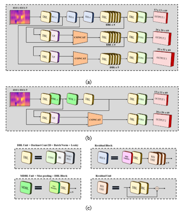Figure 14: Model architectures: a) Full YOLOv3 architecture; b) Tiny YOLOv3 architecture; c) Legend

In more details, our manuscript has described how to develop the basic and lightweight ASR as the alternative approach of the classical ASR that might be effective in certain complex spoken sentences or languages like Thai, and could be employed in many scenarios where the real-time requirement is crucial. Our data collection is juts utilized to show the specific occurrences that can be applied to our proposed strategy. By applying computer vision technique to the linguistics field, the state-of-the-art one-stage object detector, You Only Look Once, is chosen and responsible for keyword classification and localization due to its detection performances. YOLOv3 also released the lightweight and optimized version of its full architecture as Tiny YOLOv3. Since this version of YOLOv3 is appropriate for performing the real-time computing on the resource-limited platform like edge devices, we also decided to compare this version of YOLOv3 on the same task with the regular YOLOv3. The differences between the full YOLOv3 and tiny YOLOv3 structures are described on Figure 14.  The training strategy of our models are clearly explained on the following section.

7. Network Training Method

Since object detection was the supervised learning, we needed to provide the ground truth to the network. Therefore, before the training process, each target keyword on the MFCC feature images of the training set needed to be manually labeled. In this phase, the LabelImg tool has been used because the YOLO annotation format has already been provided. Consequently, the XML file according to each MFCC image would be generated to indicate the necessary labeling information for the network training step. In detail, the actual labeling steps were holding the mouse cursor, framing the target keyword region, and then double-clicking to identify the corresponding keyword class. The YOLO annotation format in XML file was composed of class index, the quotient of x-coordinate of the bounding box’s center and the image width, the quotient of y-coordinate of the bounding box’s center and the image height, the quotient of the bounding box width and the image width, and the quotient of the bounding box height and the image height. Due to the fact that the keyword in the MFCC feature image had the unique pattern, then it is possible to readily separate the specific keyword region from the uniform background noise region. The example of keyword labeling was described in Figure 15.

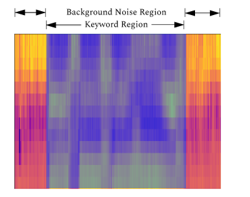Figure 15: The example of keyword labeling.

      The training platform in this article were carried out on the desktop PC (OS:Ubuntu 16.04LTS system, RAM: 16 GB, GPU: Nvidia GeForce GTX 1070Ti, CPU: Intel Xeon 8 cores). Both regular and tiny version of YOLOv3 were trained under the Darknet framework then the training results were analyzed to prove that Tiny YOLOv3 performance was acceptable for the proposed method. The stochastic gradient descent algorithm was used to perform the network training. In order to start training the model, we chose the pre-trained models of the ImageNet dataset as the initial convolutional weights. By considering the training durations, the maximum number of iterations was extended and the training process would be stopped whenever the loss was low enough. We set the Batch parameter to 64 and the Subdivision parameter to 16. As a result, the batch was split into 8 mini-batches which could not only reduce the memory usage, but also accelerate the training process and also generalized the model. Next, the learning rate was chosen to be 0.001. During training, the average loss and mean average precision (mAP) could be visualized in real-time using the graph as shown in Figure 16a. The final results were shown in Table 2.

Table 2: The models’ performance of all datasets

Weights	Iterations	Loss	mean Average Precision (mAP)
Airline names
Tiny YOLOv3	49000	0.12	0.99
Full YOLOv3	21400	0.005	0.99
Numbers (0-9)
Tiny YOLOv3	50000	0.16	0.98
Full YOLOv3	34800	0.012	0.98
Frequently Asked Questions
Tiny YOLOv3	287000	0.08	0.99
Full YOLOv3	41100	0.029	0.98

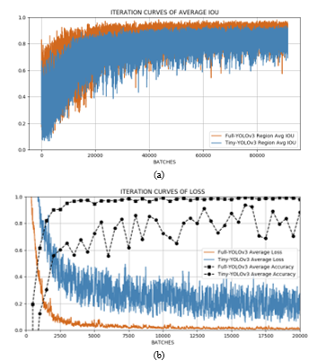Figure 16: Iteration curves: (a) Iteration curves of loss;  (b) Iteration curves of average IoU

As shown in Figure 16, although the fitting degree and the average IoU value of the full version of YOLOv3 was superior compared with the tiny version of YOLOv3, the light-weight version of YOLOv3 appeared to have well-enough training result and could be employed for further experimental evaluations.

8. Experiment and Analysis of Results

In order to investigate the true performance of the finally trained YOLOv3 weights, we considered using the unseen MFCC feature images extracted from the extra recorded voices of 20 individuals (10 males, 10 females) who didn’t present in the prior training lists. This experiment was conducted to represent the airport use case of our proposed approach in real life. Whether planning to fly locally or internationally, an airport is always the first priority to asking for the flight information and useful navigation suggestion. From that point of view, we then proposed the autonomous information providing system that could respond to the frequently asked questions (FAQs) of the flight information from the passengers based on the flight number they told in real time. This service might provide passengers all the information they need on their flight only with their voice. This service is therefore straightforward and convenient to use, and additional services such as self-check-in can be integrated and the time and costs of congested and crowded airports can be reduced. For the first task, the automatic speech recognition system was used for detecting the airline names. Then, the 1-to-4-digit numbers would be recognized by the second task. The flight number was then confirmed by the combination of airline name and airline number. In Figure 17, we illustrated some examples of this task. Firstly, our proposed system expected the airline name which was “การบินไทย” (kan – bin – thai) or Thai Airways (TG) on the upper left of figure. Next, it would ask for airline number which was “ห้า สี่ สาม เจ็ด” (haa – see – saam – jet) or 5-4-3-7 on the upper right of figure. The flight number, TG5437, was then generated by combining these two inputs which showed on the ticket.

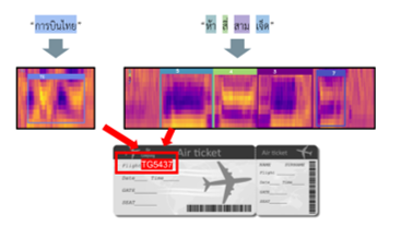Figure 17: The example of the flight number recognition

Next, the third task was responsible for answering the frequently asked questions (FAQs) according to the provided passenger flight number. The third task example was described in Figure 18 respectively. In Figure 18, we presented some tasks from all seven the frequently asked questions (FAQs) categories of the flight information from the passengers. In the left side of figure, the input interrogative sentence “ราคาเท่าไหร่?” (la-ka-tao-lai) meant “how much is a ticket?”. In this sentence, it contained two keywords that related to airflare category (described in Figure 13) which were ราคา (PRICE) and เท่าไหร่ (HM), then the system responded with all available ticket prices. Next, in the right side of figure, the input interrogative sentence “เช็คอินที่ไหน?” (check-in-tee-nai) meant “where is my check-in gate?”. This sentence contained one keyword which was เช็คอิน (CHECKIN), thus the system knew that it related to gate checking question and performed the location guidance service.

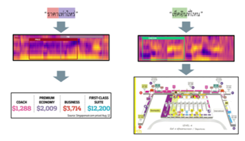Figure 18: The example of the FAQs recognition

In this experiment, Precision, Recall and F1 score were used as the evaluation metrics. Precision is the proportion of the amount of correctly detected keywords over the entire number of detected keywords. Recall is the proportion of the amount of correctly detected keywords over the entire number of keywords in the experiment set. The F1 score is the harmonic mean of Precision and Recall at particular thresholds. The calculation formulas were shown in Equations (17)-(19).

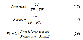Specifically, TP, or True Positive, indicates the amount of correctly detected keywords. TN, or True Negative, indicates the amount of correctly detected backgrounds. FP, or False Positive, indicates the number of incorrect detections. FN, or False Negative, indicates the number of missed detections.

      The full and tiny version of YOLOv3 were trained and tested separately on three different tasks. Airline name detection was the simplest task and the FAQs recognition was the most challenging task. In detail, Airline name detection required just the one utterance, which might contain just one name, and so resulted in high precision and recall in both tiny and full YOLOv3 model. The next challenge was that of the airline number which required the sequence of 1-to-4-digit numbers, thus it could be seen that the accuracies of both models were slightly dropped. The last assignment was the most difficult, which the input sentence could be varied depending on the speaker experiences. To tackle this challenge, we used the keyword spotting idea to search for only the related terms we defined and categorized. As a result, it seemed that the detection performances of both networks have declined dramatically yet remained over 0.6. The detection threshold and IoU in this experiment were set at 0.20 and 0.50 respectively. The true positive, false positive, false negative, precision, recall, and F1-score results for all test samples were summarized in Table 3. The comparison of the F1-score of both full and tiny YOLOv3 on three different tasks could then be visualized in Figure 19. The test results showed that the first task was highly sensitive for both models, airline name detection, which was the easiest task and then experienced poor detection result on the last task, the FAQs recognition task, the hardest task as we mentioned previously. By compared with the full version of YOLOv3, the light-weight and simplified vision of YOLOv3, so-called tiny YOLOv3, could receive the comparable performance and could unusually outperform in terms of Recall by almost 0.1 on the second task. To clarify the poor performance of both models on the third task, the FAQs recognition task, two potential reasons were given as following. First, the number of classes was doubled in comparison with the first and second tasks and the non-keyword parts might be included in a spoken sentence. Second, the input MFCC feature dimension may vary by the length of the sentence and the words can be compressed when the input images have been scaled, leading to feature loss and false negative.

Table 3: Performances of both models on testing dataset

Weights	IoU = 0.50, Threshold = 0.20
	TP	FP	FN	Precision	Recall	F1
Airline names
Full YOLOv3	91	2	1	0.978	0.989	0.984
Tiny YOLOv3	90	6	0	0.938	1	0.968
Numbers (0-9)
Full YOLOv3	192	39	70	0.831	0.733	0.779
Tiny YOLOv3	221	58	48	0.792	0.822	0.807
Frequently Asked Questions
Full YOLOv3	121	39	83	0.756	0.593	0.664
Tiny YOLOv3	108	61	74	0.639	0.593	0.615

     Based on the detection performances shown in Table 3, the average F1-score of the full and tiny YOLOv3 from three different tasks were 77.54% and 77.23% respectively. In terms of localization performance using the same box labels, the tiny YOLOv3 boxes seemed to have slightly shifted due to the simpler model architecture, which was shown in Figure 20, however, it was not affected the keyword detection proficiency. In conclusion, the experiment results showed that the tiny YOLOv3 could perform well enough and have competitive results with the full YOLOv3.

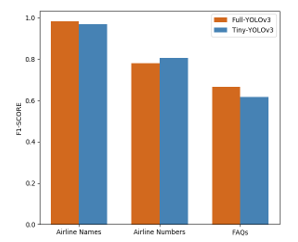Figure 19: The comparison of three task detection results

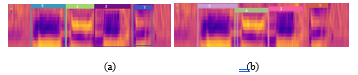Figure 20: The comparison of the localization accuracy:  a) Full YOLOv3; b) Tiny YOLOv3.

Furthermore, in order to test the model robustness, we injected the white noise with the relative amplitude  from 0.1 to 0.4 to each of the audio files using the Audacity software. In accordance with the white light which contains all wavelengths with equal intensity of the visible spectrum, white noise also contains the equally distributed energy in all audible frequencies resulted in a steady humming sound. The F1 score and accuracy measured after increasing the white noise intensity, which belonged to the regular and tiny YOLOv3 were shown in Figure 21, in which the y-axis was the measure and the x-axis was the intensity ( ) of the white noise added to the audio files.

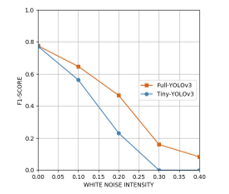Figure 21: The performances of the full and tiny YOLOv3 when injecting the background noise.

      It could be seen from Figure 22 that the full YOLOv3 model had the better adaptability than the tiny YOLOv3 to the noisy environment. Although the higher degrees of noise intensity could significantly degrade the model performances, the F1-score above 0.65 could still be obtained by both models when the variances of the white noise were below 0.05.

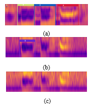Figure 22: The comparison of the detection results:

1. a) =0.1; b) =0.2; c) =0.3.

9. Conclusions and future work

This study provided the alternative approach for the automatic speech recognition (ASR) was proposed to detect Thai keywords in the spoken sentence. We next proposed the three separate real-world tasks to examine our model detection capabilities. The tasks were different in terms of difficulty, ranging from the standard test that just recognized the Thai Airway names, to the most difficult assignment that detects the specific keywords in the frequently asked questions (FAQs) using the keyword spotting technique. The core methodology is based on the Mel-frequency cepstral coefficients (MFCC), which is chosen as the feature extraction for the speech signal, because this technique artificially implements the behavior of the human hearing mechanism based on the usage of the non-linear frequency scale of the real human, so it results in the parametrically resemblances between the extracted vectors and human sense of hearing. Then the state-of-the-art convolutional neural network object detector, You Only Look Once (YOLO), was performed as the keyword localizer and classifier. Due to the requirements of real-time speed and high accuracy of the ASR system, the tiny version of YOLOv3, which was the simplified and light-weight version of YOLOv3, was evaluated and compared with the regular version using the precision, recall, and F1-score to verify the feasibility and superiority. From the experiment, the F1-score of the full and tiny YOLOv3 from three different tasks were 77.54% and 77.23% respectively. To conclude, tiny YOLOv3, with the lower computational time and comparable detection accuracy compared to the regular YOLOv3, was proven to meet the ASR requirements and was the most suitable model for using in the low resource platforms.

      Thai ASR was still the interesting and challenging topic because of the morphological richness of Thai language and the difficulties in developing Thai ASR model using the traditional technique. The YOLOv3 was applied to the keyword detection. Nevertheless, the experimental results drew back some further applications and additional improvements.

1. Compared with the results on the first and second task, the poor result on the third task told that the dataset should to be increased to produce higher performance.
2. To increase the model robustness to the background noise, injecting noise into dataset and trained together with the original dataset should be useful.
3. This work only proposed the Thai ASR application in the real-world airport scenario. Therefore, the research of the same basis should be increased to extend the application or investigate the new approaches.

Conflict of Interest

The authors declare no conflict of interest.

1. K. Sukvichai, C. Utintu, and W. Muknumporn, “Automatic Speech Recognition for Thai Sentence based on MFCC and CNNs,” 2021 Second International Symposium on Instrument, Control, Artificial Intelligance, and Robotics (ICA-SYMP), 2021. doi:10.1109/ica-symp50206.2021.9358451
2. H. Thaweesak Koanantakool, T. Karoonboonyanan, and C. Wutiwiwatchai, “Computers and the Thai Language,” IEEE Annals of the History of Computing, 31(1), 46-61, 2009. doi:10.1109/mahc.2009.5
3. T. Pathumthan, ‘‘Thai Speech Recognition Using Syllable Units,’’ master’s thesis, Chulalongkorn Univ., 1987.
4. S. Suebvisai, P. Charoenpornsawat, A. W. Black, M. Woszczyna, and T. Schultz, ‘‘Thai Automatic Speech Recognition,’’ Proc. IEEE Int’l Conf. Acoustics, Speech, and Signal Processing (ICASSP), 2005. doi:10.1109/icassp.2005.1415249
5. I. Thienlikit, C. Wutiwiwatchai, and S. Furui, ‘‘Language Model Construction for Thai LVCSR,’’ Reports of the Meeting of the Acoustic Soc. of Japan, ASJ, 131-132, 2004.
6. M. Woszczyna, P. Charoenpornsawat and T. Schultz. “Spontaneous Thai Speech Recognition.” The Ninth International Conference on Spoken Language Processing Multimodal Technologies, Inc. Carnegie Mellon University, Australia, 2006.
7. S. Kasuriya, V. Sornlertlamvanich, P. Cotsomromg, S. Kanokphara, and N. Thatphithakkul, ‘‘Thai Speech Corpus for Speech Recognition,’’ Proc. Int’l Conf. Int’l Committee for the Coordination and Standardization of Speech Databases and Assessments (O-COCOSDA), 105-111, 2003.
8. S. Tangruamsub, P. Punyabukkana, and A. Suchato, “Thai Speech Keyword Spotting using Heterogeneous Acoustic Modeling,” 2007 IEEE International Conference on Research, Innovation and Vision for the Future, 253-260, 2007. doi:10.1109/rivf.2007.369165
9. P. Khunarsa, J. Mahawan, P. Nakjai, and N. Onkhum, “Nondestructive Determination of Maturity of the Monthong Durian by Mel-frequency Cepstral Coef?cients (MFCCs) and Neural Network,” Applied Mechanics and Materials, 885, 75–81, 2016. doi:10.4028/www.scientific.net/amm.855.75
10. Y. Segal, T. S. Fuchs, and J. Keshet, “SpeechYOLO: Detection and Localization of Speech Objects,” Interspeech 2019, 2019. doi:10.21437/interspeech.2019-1749
11. G. Chen, C. Parada, and G. Heigold, “Small-footprint Keyword Spotting using Deep Neural Networks,” 2014 IEEE International Conference on Acoustics, Speech and Signal Processing (ICASSP), 4087–4091, 2014. doi:10.1109/icassp.2014.6854370
12. J.R. Rohlicek, W. Russell, S. Roukos, and H. Gish, “Continuous Hidden Markov Modeling for Speaker-independent Word Spotting,” International Conference on Acoustics, Speech and Signal Processing (ICASSP), 627–630, 1990. doi:10.1109/icassp.1989.266505
13. D. Grangier, J. Keshet, and S. Bengio, “Discriminative Keyword Spotting,” Automatic Speech and Speaker Recognition, 173–194, 2009. doi:10.1002/9780470742044.ch11
14. S. Fernández, A. Graves, and J. Schmidhuber, “An Application of Recurrent Neural Networks to Discriminative Keyword Spotting,” Artificial Neural Networks – ICANN 2007, 220–229, 2007. doi:10.1007/978-3-540-74695-9_23
15. T. Sainath and C. Parada, “Convolutional Neural Networks for Small-Footprint Keyword Spotting,” 2015.
16. D. Namrata, “Feature Extraction Methods LPC, PLP and MFCC in Speech Recognition,” International Journal for Advance Research in Engineering and Technology (ISSN 2320-6802), 1, 2013
17. R. Ranjan, A. Thakur, “Analysis of Feature Extraction Techniques for Speech Recognition System,” International Journal of Innovative Technology and Exploring Engineering (IJITEE) (ISSN 2278-3075), 8. 2019
18. Z.Q. Zhao, P. Zheng, S.T. Xu, and X. Wu, “Object Detection with Deep Learning: A Review,” IEEE Trans. Neural Networks Learn. Syst., 1-21, 2019.
19. R.L. Galvez, A.A. Bandala, E.P. Dadios, R.R.P. Vicerra, and J.M.Z. Maningo, “Object Detection Using Convolutional Neural Networks,” TENCON, 2018. doi:10.1109/tencon.2018.8650517
20. H. Jiang and E. Learned-Miller, “Face Detection with the Faster R-CNN,” 2017 12th IEEE International Conference on Automatic Face & Gesture Recognition, 2017. doi:10.1109/fg.2017.82
21. Z.-Q. Zhao, H. Bian, D. Hu, W. Cheng, and H. Glotin, “Pedestrian Detection Based on Fast R-CNN and Batch Normalization,” Lecture Notes in Computer Science, 735-746, 2017. doi:10.1007/978-3-319-63309-1_65
22. R. Girshick, “Fast R-CNN,” 2005 IEEE International Conference on Computer Vision (ICCV), 2015. doi:10.1109/iccv.2015.169
23. K. He, X. Zhang, S. Ren, and J. Sun, “Spatial Pyramid Pooling in Deep Convolutional Networks for Visual Recognition,” IEEE Trans. Pattern Anal. Mach. Intell., 37(9), 1904–1916, 2015.
24. J. R. R. Uijlings, K. E. A. Van De Sande, T. Gevers, and A. W. M. Smeulders, “Selective Search for Object Recognition,” International Journal of Computer Vision, 104(2), 154–171, 2013. doi:10.1007/s11263-013-0620-5
25. S. Ren, K. He, R. Girshick, and J. Sun, “Faster R-CNN: Towards Real-Time Object Detection with Region Proposal Networks,” IEEE Transactions on Pattern Analysis and Machine Intelligence, 39(6), 1137-1149, 2017. doi:10.1109/tpami.2016.2577031
26. T.-Y. Lin, P. Doll ? ar, R. B. Girshick, K. He, B. Hariharan, and S. Belongie, “Feature Pyramid Networks for Object Detection,” 2017 IEEE Conference on Computer Vision and Pattern Recognition (CVPR), 2017. doi:10.1109/cvpr.2017.106
27. W. Liu, D. Anguelov, D. Erhan, C. Szegedy, S. Reed, C.-Y. Fu, and A. C. Berg, “Ssd: Single Shot Multibox Detector,” in Lecture Notes in Computer Science, 21-37, 2016. doi:10.1007/978-3-319-46448-0_2
28. J. Redmon, S. Divvala, R. Girshick, and A. Farhadi, “You Only Look Once: Unified, Real-Time Object Detection,” 2016 IEEE Conference on Computer Vision and Pattern Recognition (CVPR), 2016. doi:10.1109/cvpr.2016.91
29. C. Szegedy, W. Liu, Y. Jia, P. Sermanet, S. Reed, D. Anguelov, D. Erhan, V. Vanhoucke, and A. Rabinovich, “Going deeper with convolutions,” 2015 IEEE Conference on Computer Vision and Pattern Recognition (CVPR), 2015. doi:10.1109/cvpr.2015.7298594
30. M. J. Shafiee, B. Chywl, F. Li, and A. Wong, “Fast YOLO: A Fast You Only Look Once System for Real-time Embedded Object Detection in Video,” Journal of Computational Vision and Imaging Systems, 3(1), 2017. doi:10.15353/vsnl.v3i1.171
31. J. Redmon and A. Farhadi, “YOLO9000: Better, Faster, Stronger,” 2017 IEEE Conference on Computer Vision and Pattern Recognition, 7263-7271, 2017. doi:10.1109/cvpr.2017.690
32. J. Redmon and A. Farhadi, “YOLOv3: An incremental improvement,” arXiv preprint arXiv:1804.02767, 2018.

(Click Here)