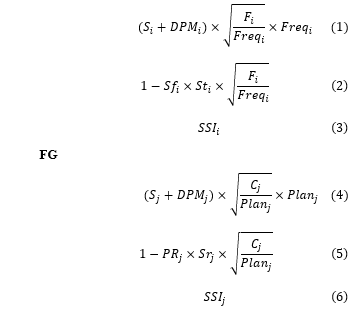
Segmentation of Stocks: Dynamic Dimensioning and Space Allocation, using an Algorithm based on Consumption Policy, Case Study

Adv. Sci. Technol. Eng. Syst. J. 6(4), 306–319 (2021);
 DOI: 10.25046/aj060434
This paper addresses the stock management aspect. Through this work, we provide a dynamic model of dimensioning and allocation of stocks to storage location for the automotive industry field. This model takes into consideration all constraints of the supply chain (24 constraints) from the suppliers passing by production, storage up to customer delivery and transport. At the end of this paper we will be able to specify the stock replenishment policy, particularly the definition of stock alerts (minimum, nominal, maximum) in quantity and days of stock, in space occupied, and in financial value. These stock thresholds will be integrated in material resource planning, storage allocation procedure and financial budget follow-up. The tool developed is decision-making support for logisticians. The algorithm proposed has solved a real instance and ensure a balanced stock fill rate (99%) in 1200 seconds.
1. Introduction
In every supply chain, the total costs that affect the logistic cost center are very high compared to all production costs. This has a direct impact on companies’ margin, and therefore, on the competitiveness of the products in the market knowing that a super high selling price cannot be accepted by all customers. In this context, companies are trying to set a demarche to control its logistics costs. The general framework of this work concerns a key element for the success of this demarche; we are talking about the immobilized cash (stocks) as well as the charges related to the surface occupied by these stocks. Inventories are the basic and main logistical data for making decisions, which can affect the operational, tactical, and sometimes strategic level. Moreover, defining a replenishment policy is fixing a minimum, average, and maximum thresholds, this implies the necessary surface area and the allocation of products to the available storage surface. The main goal is to guarantee cost control, align with budget and at the same time simplify and streamline the internal physical flow. Therefore, inventory management becomes a compulsory.
In the literature, stock management arouses the interest of researchers and manufacturers who have defined procurement policies for all contexts and types of products. In this extended paper of research, originally presented in the 5th international conference on logistics operations management (GOL’20) [1], we will define, by considering the constraints of logistics management, a dynamic stock model which will be used to define stock thresholds and serves as a decision support tool and facilitate the allocation of products in the warehouse. We will define the minimum and maximum stock alarms as well as the corresponding storage area in order to better manage both space and the cash of the company and to follow the perspectives announced in the conference paper presented in the 5th international conference on logistics operations management (GOL’20), regarding the storage location assignment problem which can be modeled as a bin packing problem based on segmentation phase results.
The rest of this article will be organized as follows: we will mention different stock policies in the state of the art. Then, we will detail the constraints of logistic management which formulate our problem of stock policy definition in addition to the assignment of stocks demarche, develop this model on Excel VBA. Finally, a real case study from an industrial background will be studied (Moroccan automotive company).
State of art
The stock management in a literature point of view depicts a multitude of replenishment policies. The most addressed are the reorder point methods (Q, R) (figure 1, part 1 taken from [2]), this demarche assumes that within a lead-time of a product, the quantity ordered should be equal to the total quantity consumed. The second method was introduced by [3] and controls stocks through up to level ordering intervals (T, S) (figure 1, part 2 taken from [2]), the Third method defines the economic order quantity (EOQ) (figure 1, part 3) as part of Wilson model for inventory management [4] considering the ordering and holding cost. Supposing that the ordering cost and delivery time is constant, moreover, the minimum stock alert is considered null, and the maximum stock that can be reached is equal to the EOQ.
There are other policies, based on the ECR: efficient consumer response. This model proposes a collaborative policy in an efficient way between the manufacturers and distributors to boost the gains and achieve high level of productivity from the supplier up to the consumer among of them we can address:
Continuous replenishment planning (CRP), it is a base that supports the efficient consumer response, which refers to a program that triggers the production and the flow of a product through the supply chain as soon as an identical product have been purchased by the end consumer. As shown by [5] brings varying benefits in terms of inventory cost savings.
SSM (GPA in French) which means the shared supply management and includes two types: vendor managed inventory (VMI) with or without consignment, the co-managed inventory (CMI).
The consignment stock (CS) which is an innovative approach to manage inventories in which the vendor removes his inventory and maintains a stock of materials at the buyer’s plant. The reference [6] treats the consignment stock policy considering economical and logistics constraints and define the minimum and maximum stock levels of a vendor managed inventory.
We find also the deterministic and stochastic demand assumption, and stock out assumptions if we lose the customer or there is a stock out cost to pay or assume.
To the best of our knowledge, none of the models addressed in the literature, have treated the constraints of inventory management that we will approach all together.
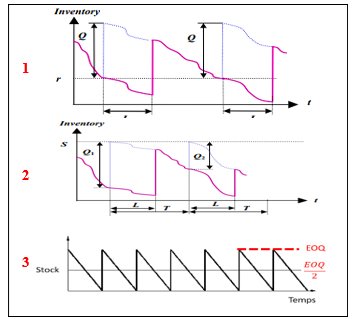 Figure 1: Part 1 (Q,R) policy, Part 2 ( T.S) policy, Part 3, (EOQ) policy
Problematic
In an automotive industry environment, between the most uncertain goals to attain we can cite inventory objective level; a supply manager is facing difficulties to determine the policy of procurement in such an uncertain environment. Defining the minimum and maximum replenishment level to ensure production and customer needs, and meet the financial targets set by the top management. This target is calculated in function of the turnover and working days and without integrating the real logistical constraints. To avoid the problem of shortage, the stock managers are obliged to put more and more days in stock, for most cases in a non-efficient way. The model we propose will stands for a decision making support tool that assists stock managers, to determine fixed and variable stock parameters: in order to calculate the minimum and maximum alerts of stock in function of the EOQ. These parameters will be integrated in the material resource planning (MRP) which involves the calculation of requirements, but in an efficient and dynamic way, considering also the main variables impacting the EOQ : type of stocks, the daily average consumption and other vital parameters such as: transit time, minimum ordered quantity. Then assigning the defined stock targets to the storage location areas.
Objectives
By means of this research, we intent to:
• Define the minimum, nominal, maximum stock alerts, in value and in quantity and in days of stock taking into account the various parameters of stock.
Define the correct storage area for products in the warehouse in function of the stock alerts defined: dynamic storage.
Assign products to storage location by maximizing the net surface used while minimizing the distance between the same families of product (multi-purpose).
Check the correspondence of the defined stock with the available surface.
Guarantee the Fluidity of goods through the different process of the supply chain.
Segmentation of stock: dynamic model
4.1. Constraints of management
In a supply chain, the flow from the supplier up to the customer involves many parameters of management specific to each stage or part of this chain; these parameters directly affect the policy of stock management and make it complicated to define.
If we take the procurement phase as an example, the ordered quantity by the purchaser must abide by the supplier terms defined in the supplier schedule agreement, particularly the minimum batch supply. The ordered quantity should be greater to the minimum batch defined by the supplier to maintain the price defined in the contract; otherwise, a new price will be applied because of the new batch order which will be greater than the defined one. In the other hand, if the gap between the two quantities is really huge compared to the weekly average consumption, the purchaser have to assume the gap in stock even if it will not be consumed immediately, moreover, he has to reserve a space for this gap while waiting for its consumption.
This kind of constraints can have less impact in some cases, for example if the daily average consumption is equal or is a multiple of the supplier batch size, in this case we can order only the required quantity and respect the targeted days of coverage set by the logistic manager. To deal with these constraints and to define the stock management policy, we must start by listing and classifying those constraints all over the supply chain, then taking them into consideration while dimensioning the stocks.
The identified constraints in a supply chain while managing the procurement or the sale of products are defined below and was collected from the industrial sector (several meetings were conducted with logistic managers, engineering pilots, purchasing teams were done in order to regroup all the constraints):
For the raw materials we define:
Packaging: define the parts in one package, it can be expressed in Kilograms, Meters or Pieces; this data could be found in the logistic contract of each product.
Batch supply: minimum quantity ordered from a supplier with a normal price.
Transport Frequency: procurement delivery frequency and represents the number of inbounds in a period (week, two weeks, one month) divided by the period expressed in days.
Scrap Rate: rejection due to the process (production) and all rejected parts by quality controllers
DPM: defective parts per million due to the supplier quality of delivered pieces.
Supplier service rate in full: quantity of parts received compared to the ordered quantity in the firm horizon.
Supplier service rate on time: quantity of supplies on time divided by total quantity supplied in a specific period.
Production Reliability rate: the volume declared in production divided by total volume scheduled by logistics.
Daily average consumption: average consumption of a product due to production and related to the explosion of bill of materials.
Supplier Firm lead time: number of working days separating the day following the order and the day of the delivery.
Supplies Frequency: the procurement program update frequency
Supplier Transit Time: duration in working days between the supplier’s plant and the customer point of delivery.
Price: unit price of the product in monetary value.
Stock for Specific issues: safety stock resulting of a managerial Decision or imposed by the supply policy.
Packaging details: dimensions authorized stacking level.
For the finished goods we define:
Packaging: define the parts in one package.
Minimum production batch size: minimum quantity to launch in production lines.
Delivery Frequency: customer delivery frequency, it represents the number of trucks loaded to deliver in a period divided by the period expressed in days.
Rejection Rate and Scrap rate: scrap rate at the end of production and rejected parts following a quality control.
Production Reliability Rate: the ratio between the volumes produced and the planned volumes.
Service rate on time in full: the ratio between deliveries on time and the total expected deliveries on a specific period.
Customer DPM: Defective parts per million delivered to the customer.
Customer variability: maximum tolerated variability of delivery instructions (firm orders compared to forecast )
Daily average deliveries. : the mean daily deliveries.
Customer firm lead time: number of working days separating the day following the release of orders, and the expected day of the delivery.
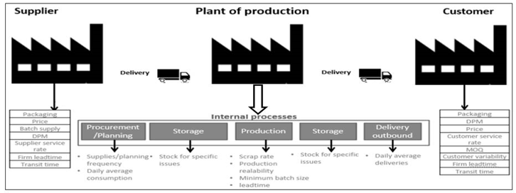 Figure 2: Constraints of management of products in a supply chain
Planning frequency: the master Production Schedule update frequency.
Production lead time: time between the Raw Materials out of stock and Finished Goods produced. Must be expressed in working days.
Transit time: the time between the warehouse and the agreed delivery place.
Stock for specific issues: safety stock due to management or customer decision.
Price: unit price in monetary value.
4.2. Proposed model of stock
The operating stocks in the model proposed are defined as follows:
Static stock
For raw materials / finished goods:
The stock covering the non-respect of the production schedule.
The stock covering the non-quality, non-compliance, rejects.
The defined stock for specific issues: decision of top management committee or customer.
Dynamic stock
For raw materials:
The stock due to deliveries, in function of supply delivery frequency.
The stock covering the gap between the order batch and the delivery frequency in case they are not synchronized.
The stock due to variability covering the non-respect of the production schedule.
For finished goods:
The stock due to deliveries, which depends on the customer delivery frequency.
The stock covering the gap between the production schedule and the delivery frequency in case they are not synchronized.
The stock covering the variability of customer orders.
Stock alerts
Minimum stock: stands for the stock related to total service rate and quality level, in addition to the stock for specific issues. This stock includes internal constraints related to both production and quality processes. It will integrated in the master production schedule MPS and supply program SP as the minimum alert to launch either the replenishment of raw materials, or production orders to maintain the level of stock for finished goods.
Nominal stock: stock covering all the constraints mentioned before and ensures the availability of material for production, the total stock hovers around this nominal stock.
Maximum stock: represents the nominal stock added to stock due to the supplier batch size (for raw materials) and production batch (for finished goods) in addition to the stock due to variability. This maximum stock will be integrated also in the MPS/SP program and stands for the upper limit of total stock. This maximum stock could be reached and tolerated by the top management in these two cases :
While receiving a new inbound batch (new reception).
Before an outbound delivery (stock assigned to the temporary preparation area/ Bin waiting to be loaded in customer truck).
Dynamic surfaces:
Dynamic surfaces have a direct link with the minimum, nominal and maximum stock, and are generated to follow the variability of these stocks:
Minimum surface: stands for the minimum space that would accommodate the minimum stock defined expressed in handling units (number of pallets for example), integrating the unit area of one handling unit and the possible stacking level as well as the type of storage (flat or shelving).
Nominal surface: stands for the nominal space that would accommodate the nominal level of stock defined expressed in handling units, integrating the unit area of one handling unit and the possible stacking level as well as the type of storage (flat or shelving).
Maximum surface: stands for the maximum area that would accommodate the maximum stock defined expressed in handling units, integrating the unit surface of the handling unit and the number of stacking levels as well as the type of storage space (flat, which means massive or shelving using metallic structures).
Storage location allocation:
The problem of allocating materials to the storage location area can be modeled as a task assignment problem as schematized below:
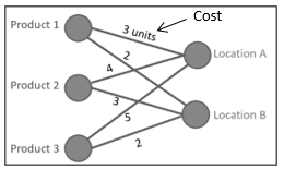 Figure 3: modeling of task assignment problem
As shown in the figure above, we will assign products (represented with handling units) to the storage location, which is divided to sub storage location named bins. Our problem can also be considered as a bin packing problem. It is about finding the most economical storage possible for a set of items into bins.
In our case, it is about finding the closest optimal assignment for a set of products that are assigned to storage location. Respecting lean flow directives (raw materials and finished goods should be stored separately to avoid flow congestion). The storage locations will be represented by boxes (Bins) and the products will be represented by items. To solve this NP hard problem we will use tree dimensional Bin packing algorithm, and to improve results we will pair the bin packing algorithm to an algorithm of list (first fit decreasing problem [7].
The table below summarizes the analogies between our assignment problem and the core model of bin packing problem modified from [8] considering the 3 dimensions and the constraints related to our context :
Table 1: Analogies between bin packing and our problem
| Criteria | Bin packing problem | Stock allocation problem |
| Data | Article | products |
| Bin | Storage location | |
| Volume of the article | Dimensions of the product | |
| Objective function | Assigning items to bins | Assign stocks to volume
|
| Constraints | The volume capacity of the bin | The volume of the storage location |
| Objective | Minimize the number of bins used | Minimize the volume used
|
| Other | Compatibility constraint between raw materials and final products, they must be separated to better flow organization, and between bins and products in function of storage type |
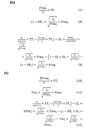
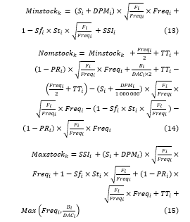
Parameters and Equations
Notation
Table 2: Stock parameters
| Raw Materials | |
| Parts per packaging of the raw material (RM) i | |
| Batch Supply of the RM i | |
| Supply Frequency of the RM i | |
| Scrap Rate of the RM i | |
| DPM of the RM i | |
| Supplier service rate in full of the RM i | |
| Supplier service rate on time of the RM i | |
| Production Reliability rate of the RM i | |
| Daily average consumption of the RM i | |
| Supplier Firm lead time of the RM i | |
| Supplies Frequency of the RM i | |
| Supplier Transit Time of the RM i | |
| Stock for Specific issues of the RM i | |
| Price of the RM i | |
| Length of the RM i | |
| Width of the RM i | |
| Stacking level of the RM i | |
| Finished Goods | |
| Packaging of the finished good (FG) j | |
| Minimum production batch size of the FG j | |
| Delivery Frequency of the FG j | |
| Rejection Rate and Scrap rate of the FG j | |
| Production Reliability Rate of the FG j | |
| Service rate on time in full of the FG j | |
| Customer variability of the FG j | |
| Daily average deliveries of the FG j | |
| Customer firm lead time of the FG j | |
| Planning frequency of the FG j | |
| Production lead time of the FG j | |
| DPM of the FG j | |
| Stock for specific issues of the FG j | |
| Customer Transit time of the FG j | |
| Price of the FG j | |
| Length of the FG j | |
| Width of the FG j | |
| Stacking level of the FG j | |
| DAC | Daily average consumption |
| Stock alerts in quantity | |
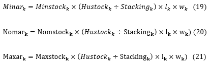
| Minimum stock of the part number k | |
| Nominal stock of the part number k | |
| Maximum stock the part number k | |
| Dynamic surface | |
| Length of the part number k | |
| Width of the part number k | |
| Number of packages in part in a handling unit for the part number k | |
| Authorized stacking level for the part number k | |
| Minimum surface for the part number k | |
| Nominal surface for the part number k | |
| Maximum surface for the part number k | |
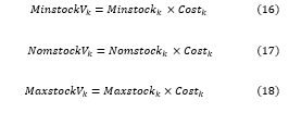
| Stock alerts value | |
| Minimum stock of the part number k | |
| Nominal stock of the part number k | |
| Maximum stock the part number k | |
| Unit cost of the part number k | |
The graphic bellow synthetizes the static and dynamic stocks taken into consideration in our model:
Dynamic stock: represents the level of stock made available to the planner for smoothing.
Static stock: represents the incompressible level of stock.
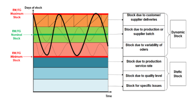 Figure 4: Static and dynamic stocks
Static stock
Dynamic stock:
 (1): Stock due to quality level.
(2): Stock due to production reliability.
(3): Stock for specific issues.
(4): Stock due to quality level.
(5): Stock due to production reliability.
(6): Stock for specific issues.
(7): Stock due to supply frequency.
(8): Stock due to production variability.
(9): Stock due to supplier batch.
(10): Stock due to delivery frequency.
(11): Stock due to customer variability.
(12): Stock due to production batch.
Stock alerts in quantity:
For RM:
Stock alerts in value:
 Dynamic surface:
 Allocation problem: bin packing model
The bin packing problem is NP hard in strong sense, this has been demonstrated using the reduction with 2-Partition, to solve medium to large instances we need to adopt heuristics developed particularly to solve this problem. The most popular heuristics in literature are first fit, Next fit and best fit, which have proven its effectiveness. The most adapted heuristic to our context is First fit, since the articles are assigned in a given order (in our case the order is in function of the daily average consumption). Then each article is placed in the first bin that can contain it.
A new box is considered only if this article does not fit in any box (considering the remaining empty volume in each box).The box remains open until the end of the execution of the algorithm, in case we engage the constraints of compatibility between articles, if an article is not compatible with a bin or an article or with another article already assigned in the current box, it will be assigned to the next box that ensure compatibility first then ensure the volume constraint contrary to the next fit heuristic where box is closed permanently if the volume of the current article cannot be contained in the box. The box is permanently closed, and it is impossible to assign a new article even if the remaining empty volume is enough to contain a new article. A new box is considered and becomes the current box. The reference [9] have proven the result of First fit:
![]()
Research in the article [10] have demonstrated that the sequential coupling of list algorithms and bin packing heuristics guarantee better results, the first fit decreasing is the one that provides the best results, at a factor 2 of the optimal as proved by the reference [2]. Our assignment problem involves the allocation of stocks (total handling units) to the storage location (divided into sub-storage locations) with a flow constraint, that the raw materials and final products should be stored separately to remain an organized physical flow. It serves as a simulation tool to check if the policy of replenishment proposed sticks with the space that we have in the warehouse considering that the layout and the storage location are already defined.
Next, we will adopt the first fit decreasing heuristic to resolve the storage location assigning problem based on the daily average consumption of the handling unit, which refers to the daily consumption of the product marked in the HU label, sorted in the descending order (the HU of high runner products will be assigned first). We will use the following formalization in addition to some modifications related to our context:
i: The index that represents the handling unit i.
j: The index that represents the storage location bin j.
S: The set of storage location bins in the warehouse.
HU: The set of handling units.
V_i: The volume occupied by the handling unit i (3D).
V_j : The volume of the bin j.
Dac_i: The daily average consumption of the handling unit i.
The decision variables are described below:
x_(i,j)={█(1,if the Hu i ϵ HU is assigned to the storage bin jϵ S@0,else )┤
C_(i,j)={█(1,if the HU i∈HU is compatible with the Bin j∈S@0,else )┤
The algorithm bellow describes the first fit decreasing algorithm adopted which is the sequential coupling of the list algorithm based on the consumption of productions and the first fit algorithm:
Algorithm 1: The principle of the first fit decreasing algorithm
Result: A_j∀j∈S
Input data:
HU, i∈{1,…,card(HU)} 〖,V〗_i ,Dac_i ∀i ∈ HU
〖S ,j∈{1,…,card(S)} ,V〗_j ,∀j∈S
C_(i,j), ∀ j∈S
Initialization:
A_j =0, the initial volume of the bin j ∀j∈ S, all bins is empty at the beginning.
〖Chart A〗_((3,card(HU))) , the chart with card (HU) columns and 3 lines that contains respectively: 〖Hu〗_i,V_i,〖Dac〗_i
〖Chart B〗_((3,Card(HU))) , the chart with 3 columns that contains: 〖Hu〗_i,〖V_i,Dac〗_i after the step of sorting.
Sort 〖Dac〗_i, ∀i∈HU in a descending order, then place them with the corresponding HU and volume in 〖Chart B〗_-
for k =1…card(HU) do
j : = 1, Assigned: = false
while (assigned= false) & j ≤ card(S)) do
if the HU 〖Chart B〗_(1,k) is compatible with the bin j (C_(〖chart B〗_((1,k)),j)=1) then
if 〖Chart B〗_((2,k)) holds in j, (A_j+〖Chart B〗_((2,k))<V_j) then
Assign 〖Chart B〗_((1,k)) to the bin j:
x_(〖Chart B〗_((1,k)),j)=1
A_j=A_j+ 〖Tab B〗_((2,k))
Assigned: = True
j : = j + 1
end
end
End
end
Resolution method: Segmentation and assignment of stocks
The demarche of segmentation starts from the integration of input data, until the calculation of the stock alerts: in quantity, in number of packages (HU), in financial value and in square meters.
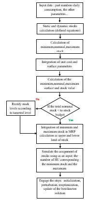 Figure 5: segmentation and assignment denmarche
The output of the segmentation demarche will be the input data for the storage location assignment demarche, the demarche starts with the initialization (input data), then engaging the first fit decreasing algorithm for the construction step (best known solution) based on the daily average consumption. Next, we will use a large neighborhood search as described below:
Step 1 (perturbation): we randomly remove handling units from bins, and randomly empty a few bins completely. Then we sort the bins in a decreasing order in function of the current volume occupied in each one A_j.
Step 2 (optimization): we select the removed HU, and reassign them into bin using a constructive heuristic, in our case we have chosen the wall building heuristic because of the flow constraints, we should place similar HUs next to each other as if we build a brick wall.
Step 3 (update of the best-known solution): if the new solution obtained is better than the best known solution, we replace the current best known solution, if not, we go back to the first step and engage a new cycle of perturbation, reoptimization.
The demarche of stock segmentation and storage location assignment is described below:
The action plan mentioned in the segmentation demarche tends to optimize six variables:
Stock delivering (adapting the frequencies of delivery to minimize the number of days of finished good stock).
Batch of production or supply (to synchronize the daily average consumption or daily average delivery).
Variability of the demand (that must be contractual).
Service Rate (of both customer and supplier).
Quality level (of both supplier and customer delivered parts) an finally the safety stock.
For the case study, we will use the script code developed by Güneş Erdoğan (CLP Spreadsheet Solver) with some modification related to our context.
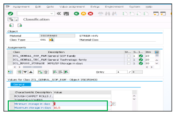 Figure 6: Master data transaction
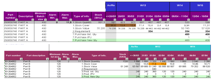 Figure 7: SP (1) and MPS (2)
Integration of alerts in MRP calculation
After the calculation of minimum and maximum alerts of stock, we integrate theme in SAP following the steps below:
Access to the transaction of master data.
Choose the classification tab.
Add the alerts of stock in the corresponding field.
This data in the classification tab will be used to run the Material Resource Planning in automatic mode (MRP job) for the frozen period or Manuel smoothing of orders for the forecast horizon.
Our alerts were integrated in the supply VBA program (SP) and Master Production Schedule VBA program (MPS) already developed by the company using EXCEL VBA. The datasheet of SP includes the following data (Figure 7):
The stock quantity and cover and value extracted from SAP.
The requirement of the part in question into the frozen and forecast horizon (named “Part A” in the figure 7).
The cover of the part in question in the end of the period (day, week).
The purchase quantity in function of the batch size or its multiples.
In each period (day, week) the quantity proposed by the system ensures that the coverage after acquisition of this quantity is between the minimum and maximum alert.
If the cover exceeds the maximum alert of stock, the system doesn’t propose any purchase quantity and jump to the next period.
The datasheet of MPS includes the following data (figure 7):
All the data mentioned in SP.
It works the same as SP, but instead of purchase quantity, we find the production quantity and instead of supplier batch size we find the production minimum size.
Limits of the proposed method
If there is an error in the input data, consequently the results will not be consistent and right.
If there is any discrepancy between the physical and the stock injected in the information system, the quantities proposed by MRP (either planned orders or purchase order) won’t ensure the coverage of stock shown in the information system.
The alerts of stock should be updated in a regular basis (every three months for example) knowing that the volumes could change in horizon forecast and the daily average consumption must follow the new volumes.
The model of assignment considers zero distance between two HUs, and the volume and number of HU are already known before engaging the solver (off-line).
Case study: Moroccan industrial compan
Segmentation of stocks
The segmentation model developed was tested in a real case study conducted using data of a Moroccan multinational company specialized in automotive parts.
We have chosen 5 references of each family to show the details of each parameters and how we can interpret the results obtained using equations and logistic parameters defined before.
After integrating the ten references in the spreadsheet developed, we obtain the result below:
After realizing the simulation with the current data we conclude the following point by family of productions
For raw materials:
To see the impact of stock due to transit time, stock to cover the frequency of delivery, and stock to covering quality of service let’s take an example of the part number A : the nominal stock is equivalent to 8.2 days this stock include also the transit time equivalent to four days.
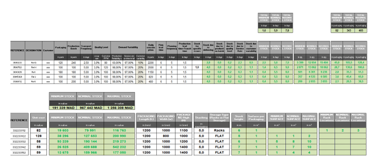 Figure 8: The datasheet of raw materials
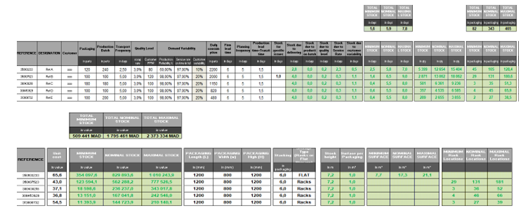 Figure 9: The datasheet of final products
This duration could be reduced if we consider local suppliers of customers, that the distance between the place of order and the place of delivery is closer. This decision could have an impact on the order cost. Then, we have 5.3 days in stock because of the frequency of delivery to customer, if there is a possibility to raise the frequency from 2 trucks to 3 trucks per week, this quantity of stock days will be largely optimized. Consequently, the overall value of stock will be optimized reducing the impact on immobilized cash. Moreover, if we have a contract with suppliers that stipulate a global service rate greater than 90%, the stock related to service rate will be improved ( currently 1,7 days). In the other hand, a minimum order quantity synchronized with daily consumption will solve many problems of returns of stocks non-consumed to the warehouse after production. This constraint was taken into consideration while developing the program under Excel VBA, so if we have a non-synchronization between these two values; this means that the resulting rate is greater than one week (generally 5 working days); the program underlines in red the minimum supplier batch. In the current simulation data, the resultant rate doesn’t exceed one week or production. Regarding the space of storage required if the storage type required is: RACK (shelving structures), the spreadsheet gives the number of modules equivalent to nominal stock for the part number A is about 2 modules. For the flat type of stock. If the storage type required is: FLAT, the spreadsheet specifies the net surface needed in square meters (for the part number B and C, the surface needed is respectively 4 and 8 square meters). For the total space needed (includes the stock net space and services aisles space), we apply a mark-up of 2.4.
Another example of optimization we found, for the reference B. The stock due to the batch supply is 1.3 days, knowing that we consume 60 parts per day, and the batch supply is 800 parts. So, if we reduce the supplier batch, we could gain 1.3 days in stock of this reference.
For the reference D, if we increase the supply frequency from 1 truck per month to 1 truck per week, we could gain 7.5 days in stock and the stock due to supply frequency will be 20.5 days. Furthermore, if we find a forwarder who can ensure the delivery in less than 18 days, for example 14 days, the stock due to supply frequency will be 16.5 stock days.
For finished goods:
The important stock for the references H,I,J,K is the stock due to the frequency of customer deliveries, that implies a stock to cover the time between two deliveries, we have 4 days for each reference, if we increase the delivery frequency for example from one truck per week to 2 trucks per week, we could gain 2 days in stock
The stock due to production service is huge for the reference G, if we oblige the production team to respect the production plan communicated by logistics, we could improve the reliability rate and gain 2.3 days in stock caused by the current production reliability rate.
Considering all this remarks, the action plan to reduce stocks should start by eliminating the important stock mentioned above. The spreadsheet also gives the corresponding space that should be revered for each reference (minimum, nominal and maximum); all these informations will serve as an input data for the assignment phase.
Assignment of stocks in storage locations
For the assignment phase, we define the following data structure according to the bin packing notation:
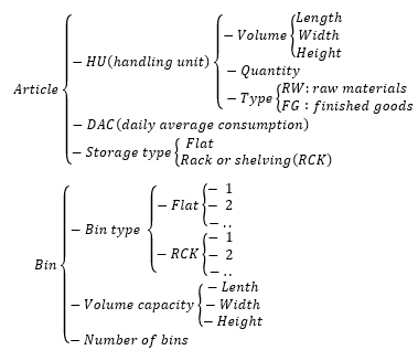 Figure 10: simulation data structure
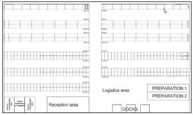 Figure 11: The layout of the warehouse
We consider the following instances:
Considering the warehouse of the company (figure 11).
The set of storage bin (Table 3).
10 reference of RW and FG (table 4 and 5) as an example. The two family of products are not compatible (can’t be stored in the same bin). Compatibility between bins and references (storage type needed).
Table 3 : The set of Bins
| Bin Type | Number of BINs | Width in meter (x) | Height in meter (y) | Length in meter(z) |
| FLAT | 10 | 28 | 6 | 1,2 |
| RCK | 10 | 28 | 6 | 1,2 |
Table 4: The set of RW references
| RW | Storage type | DAC | Number of HU | Width (meter) (x) | Height (meter) (y) | Length (meter) (z) |
| RW-1-A | FLAT | 120 | 2 | 1 | 1,1 | 1,2 |
| RW-2-B | RCK | 60 | 5 | 0,8 | 1 | 1,2 |
| RW-3-C | RCK | 400 | 33 | 1 | 1,2 | 1,2 |
| RW-4-D | FLAT | 225 | 28 | 1 | 1,4 | 1,2 |
| RW-5-E | FLAT | 116 | 11 | 1 | 1,4 | 1,2 |
| RW-6-F | RCK | 1200 | 80 | 1 | 1,1 | 1,2 |
| RW-7-G | FLAT | 700 | 56 | 1 | 1,1 | 1,2 |
| RW-8-H | FLAT | 865 | 40 | 1 | 1,1 | 1,2 |
| RW-9-I | FLAT | 923 | 21 | 1 | 1,1 | 1,2 |
| RW-10-J | RCK | 1032 | 84 | 1 | 1,1 | 1,2 |
Table 5 : The set of FG references
RW Storage type DAC Number of HU Width (meter) (x) Height (meter) (y) Length (meter) (z)
| RW | Storage type | DAC | Number of HU | Width (meter) (x) | Height (meter) (y) | Length (meter) (z) |
| FG-1-A | FLAT | 2200 | 105 | 0,8 | 1,2 | 1,2 |
| FG-2-B | RCK | 2000 | 131 | 0,8 | 1,2 | 1,2 |
| FG-3-C | RCK | 1150 | 35 | 0,8 | 1,2 | 1,2 |
| FG-4-D | RCK | 820 | 45 | 0,8 | 1,2 | 1,2 |
| FG-5-E | RCK | 480 | 27 | 0,8 | 1,2 | 1,2 |
| FG-6-F | FLAT | 640 | 50 | 0,8 | 1,2 | 1,2 |
| FG-7-G | FLAT | 500 | 42 | 0,8 | 1,2 | 1,2 |
| FG-8-H | FLAT | 140 | 64 | 0,8 | 1,2 | 1,2 |
| FG-9-I | FLAT | 980 | 99 | 0,8 | 1,2 | 1,2 |
| FG-10-J | FLAT | 655 | 83 | 0,8 | 1,2 | 1,2 |
Table 6: Simulation results
| Bin | Volume occupied | References Assigned | Number of HU assigned |
| Flat 1 | 100% | FG-9-I | 175 |
| FG-10-J | |||
| Flat 2 | 100% | FG-6-F | 175 |
| FG-1-A | |||
| FG-10-J | |||
| FG-7-G | |||
| Flat 3 | 99.94% | RW-1-A | 145 |
| RW-4-D | |||
| RW-7-G | |||
| RW-8-H | |||
| RW-9-I | |||
| Flat 4 | 54% | FG-6-F |
94 |
| FG-8-H | |||
| Flat 5 | 10.48% | RW-5-E |
13 |
| RW-9-I | |||
| Flat 6 | 0% | – | – |
| Flat 7 | 0% | – | – |
| Flat 8 | 0% | – | – |
| Flat 9 | 0% | – | – |
| Flat 10 | 0% | – | – |
| Rack 1 | 99% | FG-5-E |
173 |
| FG-2-B | |||
| FG-3-C | |||
| Rack 2 | 91% | RW-2-B |
141 |
| RW-6-F | |||
| RW-10-J | |||
| Rack 3 | 42% | RW-10-J | 61 |
| RW-3-C | |||
| Rack 4 | 38% | FG-5-E | 67 |
| FG-4-D | |||
| Rack 5 to Rack 10 |
0% |
– |
– |
We take as an example the progress of assignment of BIN 1 Flat to show how the algorithm used works:
Phase 1, 2: we place HU of the reference FG-9-I next to each other, knowing that the storage type required is “Flat”.
Phase 3: the algorithm moves to the reference FG-10-J which is compatible with the FG-9-I and also requires a flat storage type.
Phase 4, 5, and 6: the algorithm place similar items next to each other in order to form stock piles with the same references.
After engaging the assignment VBA solver developed initially by Güneş Erdoğan and modified by us for 1200 seconds and 67978 iterations, we obtain the following results:
After analyzing the simulation results, we have concluded the following points:
The number of bins used: 9 (20 in total).
Number of HU assigned: 1044 (all the HU were assigned correctly).
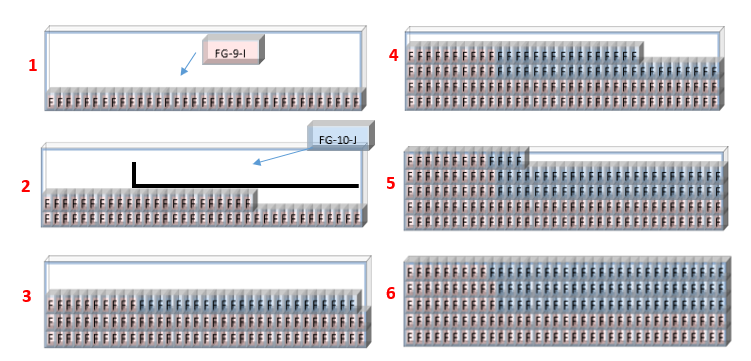 Figure 12: The assignment progress of the Bin 1 Flat
The constraints of compatibility between raw materials and finished goods have been respected; in each bin we found only one family of products; Raw materials or Finished goods but not both. This means that there will be no congestion while preparing raw materials to be transferred to the linefeed of finished goods to be transferred to preparation area.
The constraints of compatibility between the references to assign and the storage bin type (Flat or Rack) have been respected.
The filling rate of bins is maximized, where there is no constraint of compatibility.
The stocks are assigned following the physical flow, starting from the first bin, then the second, then the third… which keeps the warehouse organized.
The wall building heuristic has given good quality results, if we look at the first part of assignment progress (figure 13), we observe that the assignment is done by placing HU’s of similar articles next to each other to form the first level of stock (phase 1) then the second level (phase 2). In the third level, the heuristic moves to the article FG-10-j which is compatible with FG-9-I and place HU in the third level. Moving to the next levels, the piles formed respond to the notion: brick wall, we found a harmony of articles in each pile, which is a part of the visual management; it is easy to identify the references stored in the bin FLAT 1 as an example when we are present physically in the warehouse.
Synthesis
The spreadsheet developed defines the alerts of stocks in addition to the nominal stock in quantity, in days of stock and in monetary value for each part number. Furthermore, the required space for each reference equivalent to each alert of stock is defined considering the requested type of storage either massive or rack stock, and the tolerated stacking level. In the MRP calculation, we have integrated the upper and lower limit of stock in order to propose quantities of orders inside this interval of stock when running automatically (daily Job of MRP)
This tool facilitates the management of procurement and production planning by providing an interface including all logistics parameters throughout the supply chain impacting the EQO. The tool we have developed will facilitate the work of logistic decision-makers as it integrates the static and dynamic aspect of the stock while considering logistic management constraints. The assignment part allows to manager to check the feasibility of the stock replenishment policy defined in the segmentation phase compared to the storage locations available and the total budget authorized. Furthermore, it facilitates the management of physical flow; the spreadsheet is a logistic decision support tool. Among these advantages:
Defining adequate procurement policy and checking the alignment of the stock value calculated with the value monthly budgeted by the top management.
Defining a dynamic storage area for each item in the warehouse, if there is any change in the values of nominal stock, we anticipate the actions to be taken regarding the storage area.
Detecting the anomalies and the discrepancies regarding the various logistic parameters of supply or sale (example: supplier minimum order and daily average consumption of products) and see the impact on the number of days in stock in real time mode.
Ensuring a better interpretation of the stock constraints (FG and RM), by segmenting them into six variables, and then prioritizing the actions plan to get the optimal stock:
Stock delivering: Increase the frequency of the delivery downstream (PF) and upstream (RM).
Batch: Decrease the launches quantities (FG) and the minimum order (RM).
Variability of the demand: To master the variability of customer’s needs (FG) / to respect and smooth the production schedule (RM).
Service Rate: To respect the production schedule and follow the reliability of the customer’s loading (FG)/ Master the suppliers with the supplier service rate (RM).
Quality level: Quality action (decrease the defective parts rate…).
Safety stock: Safety stock defined following to a management decision or a customer contract decision.
Check the correspondence of the financial target defined by the top management and the stock management policy defined.
Conclusion and perspectives
The research work in our hand is very complex from a modeling point of view; the context of stocks in the industrial domain; and integrating all the constraints of operational management of raw materials and also finished goods. In terms of the initial objectives set, we successfully determine a static and dynamic model of stock calculation. Particularly, define the optimal order quantities in a detailed mathematical and algorithmic demarche. Then propose an algorithm to solve the storage location assignment problem known as NP-Hard problem and include the allocation of space to references in function of the alerts of stock defined in the segmentation phase within a Moroccan multinational company respecting the constraint of flow. Moreover, we propose a multi criteria decision tool to support decision makers in order to take decisions based on current policy of stock replenishment, and show the variables that impact the level of stocks and should be revised or negotiated. Finally, the model proposed could be replicated in any automotive industry context since it encompasses all the constraints adopted in such an exacting context. For other industries, where there is less variables we can use the same model using a relaxation approach of some constraints for each context
For further research, after solving the space allocation problem in both types rack and flat, we have detected a new constraint in the case of flat stocks. The algorithm proposed doesn’t include the order of consumption of products when assigning them in the available space; this gap provokes one of the main Muda. It includes the operations of movement of products to withdraw the requested product since all the products are stacked, and then returning the non-needed products to the stockpiles. For all these reasons, we need to solve the assignment problem of flat stock type references to the space in the warehouse considering the picking order (retrieval) of handling units while constituting stock piles and optimize rehandling operations. This problem is also NP-Hard in a strong sense and can be modeled also as a bin packing problem tree dimensions with constraints of retrieval.
Conflict of Interest
The authors declare no conflict of interest.
Acknowledgment
I would like to express my gratitude to my primary supervisor, of thesis Abdelfettah Sedqui, who guided and assisted me throughout this work of research. I would also like to thank the logistics manager of the multinational company for the data, support, and the trust. A special thanks for my wife and family who supported me during this work till the redaction of these lines. I would like to thank also the two anonymous reviewers whose constructive and helpful comments have helped considerably in improving the contents as well as the presentation of the paper.
- A. Laassiri, A. Sedqui, “Dynamic dimensioning of logistic resources: Case of stocks Moroccan multinational company,” in 2020 5th International Conference on Logistics Operations Management (GOL), 1–7, 2020, doi:10.1109/GOL49479.2020.9314755.
- M.Z. Babai, Y. Dallery, “Inventory Management: Forecast Based Approach vs. Standard Approach,” International Conference on Industrial Engineering and Systems Management (IESM05), 2005.
- G. Hadley, T.M. Whitin, Analysis Of Inventory Systems, 1963.
- F.W. Harris, “How Many Parts to Make at Once,” Operations Research, 38(6), 947–950, 1990, doi:10.1287/opre.38.6.947.
- Y. Yao, M. Dresner, “The inventory value of information sharing, continuous replenishment, and vendor-managed inventory,” Transportation Research Part E: Logistics and Transportation Review, 44(3), 361–378, 2008, doi: 10.1016/j.tre.2006.12.001.
- D. Battini, A. Gunasekaran, M. Faccio, A. Persona, F. Sgarbossa, “Consignment stock inventory model in an integrated supply chain,” International Journal of Production Research, 48(2), 477–500, 2010, doi: 10.1080/00207540903174981.
- B. Korte, J. Vygen, J. Fonlupt, A. Skoda, Le probléme du bin-packing, Springer, Paris : 475–492, 2010, doi : 10.1007/978-2-287-99037-3_18.
- A. Laassiri, A. Sedqui, “Dynamic dimensioning of logistics resources: Case of production workshop: Analogy with the problem of bin-packing Moroccan multinational company,” in 2019 International Colloquium on Logistics and Supply Chain Management (LOGISTIQUA), 1–8, 2019, doi:10.1109/LOGISTIQUA.2019.8907270.
- K. Cuthbertson, D. Gasparro, “The Determinants of Manufacturing Inventories in the UK,” The Economic Journal, 103(421), 1479–1492, 1993, doi: 10.2307/2234478.
- K.A. Cook, G.R. Huston, M. Kinney, Managing Earnings by Manipulating Inventory: The Effects of Cost Structure and Valuation Method, SSRN Scholarly Paper ID 997437, Social Science Research Network, Rochester, NY, 2012, doi:10.2139/ssrn.997437.
No related articles were found.